8 Neural Networks
Neural networks encompass a broad range of models, including deep neural networks, which have demonstrated remarkable results across various domains. These domains include image analysis (face recognition, quality control); speech technologies (virtual assistants, emotion recognition); time series analysis (investment modeling, sensor data fusion); personalized healthcare (diagnosis, drug design); personalized advertising; or autonomous vehicles. This chapter will concentrate on feed-forward neural networks, providing foundational knowledge and insights into this category of machine learning techniques.
8.1 Softmax Regression - Generalizing Logistic Regression to Multiclass Classification
In multiclass classification we have as previously a training set \(\{(\mathbf{x}^{(1)}, \mathbf{y}^{(1)}), ((\mathbf{x}^{(2)}, \mathbf{y}^{(2)}), \dots, ((\mathbf{x}^{(M)}, \mathbf{y}^{(M)})\}\) comprising pairs of inputs and corresponding labels that indicate one of \(K\) classes. The label \(\mathbf{y}^{(m)}\) is now a \(K \times 1\) binary vector encoding the label (class) of sample \(m\). For example, if we have three classes \(\{1, 2, 3\}\), and the first sample belongs to class 2 then its label will be \(\mathbf{y}^{(1)}=[0,1,0]\). This is referred to as the one-hot encoding. The goal of multiclass classification is to predict the label correctly.
Recall that logistic regression amounts to applying the logistic function on the linear combination of the inputs (the output of the linear regression). This is illustrated in Figure 8.1.
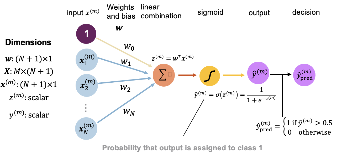
The softmax regression illustrated in Figure 8.2 generalizes this idea to multiclass classification:
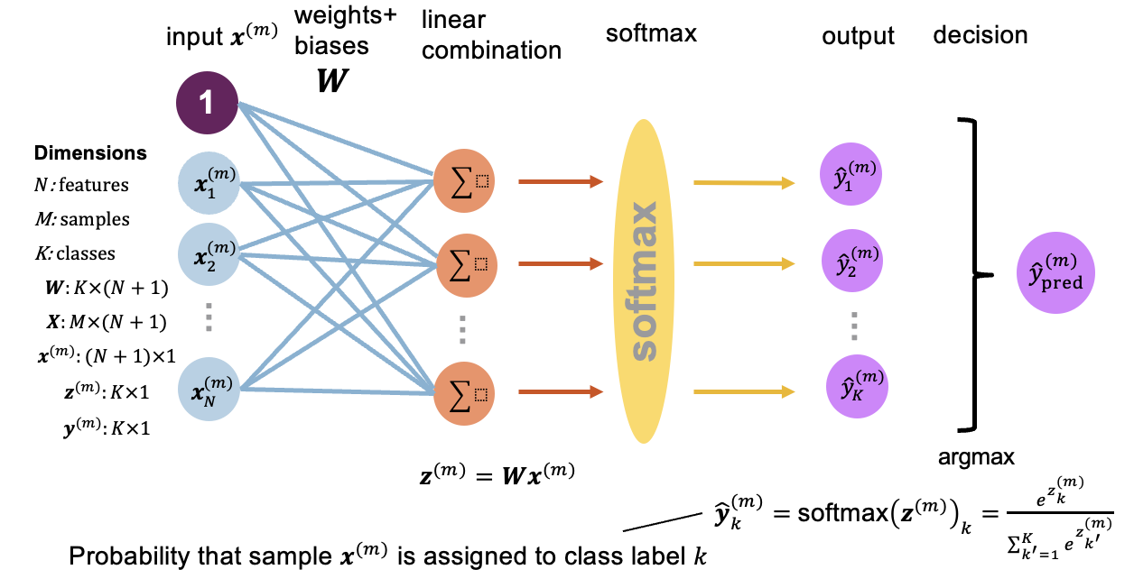
For each different class, it computes a separate linear combination of the inputs, and then applies the softmax function defined as: \[softmax(\mathbf{z})_k=\dfrac{\exp{(z_k)}}{\sum_{i=1}^{K}\exp{(z_i)}}\] to each linear combination to obtain the prediction for each class. Note that \(softmax(\mathbf{z})\) is a vector and \(softmax(\mathbf{z})_k\) is the k-th compoment of that vector. The softmax function has the nice properties of scaling the values it is applied on to the \([0,1]\) interval in a way that they sum up to one. This way they can be interpreted as probabilities or confidence of a target sample \(\mathbf{x}^{(m)}\) belonging to one of the \(K\) classes. The predicted label is then the class with the highest probability (confidence) depicted by the \(argmax\) in the image. The loss function for softmax regression is a generalization of the loss function for logistic regression and is referred to as cross entropy loss. For sample \(i\) it is defined as: \[\textrm{Loss}(\hat{\mathbf{y}}^{(m)}, \mathbf{y}^{(m)}) = - \sum_{k=1}^{K}{y_k^{(m)} \log(\hat{y}_{k}^{(m)})}\] where \(\mathbf{y}^{(m)}\) is the true label and \(\hat{\mathbf{y}}^{(m)}\) is the predicted label for the target sample \(m\). Taking the average of the cross entropy loss over all examples in the training set, we arrive at the cross entropy cost function: \[ J(\mathbf{W}) = \frac{1}{M} \sum_{m=1}^M \textrm{Loss}(\hat{\mathbf{y}}_{m}, \mathbf{y}_m). \] The model parameters are then obtained by minimizing the cross entropy cost function by gradient descent.
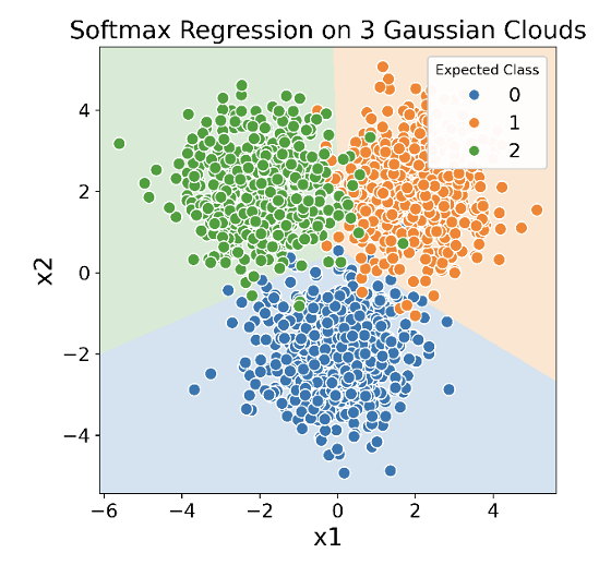
An example for three-class slassification with softmax regression is given in Figure 8.3. Note that softmax regression learns linear decision boundaries.
8.2 Feed-forward Neural Networks
In the following when we use the term neural network we will actually be referring to feed-forward neural network as defined in this section.
The main building block of a neural network is the neuron depicted below:
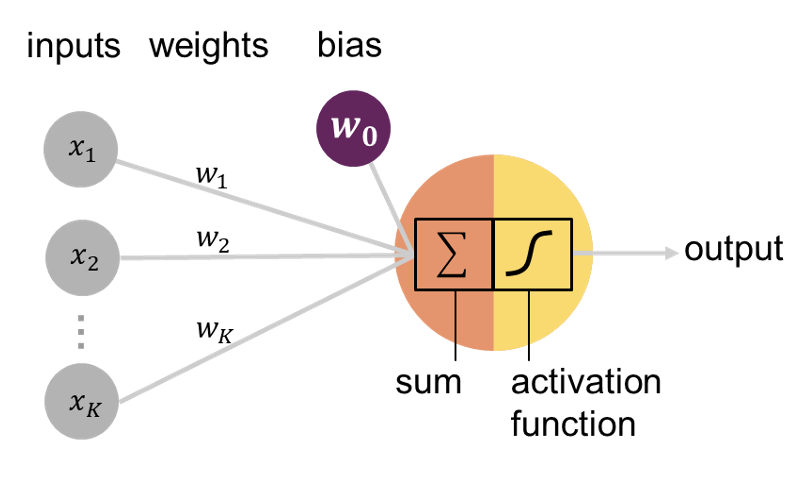
It has several inputs and one output. The output is computed by applying an activation function on the linear combination (weighted sum) of the inputs and adding a bias term (the offset) depicted in violet. This sum is also referred to as preactivation. The activation function regulates the value of the output (is it non-zero, how large its value is, …). Another way to depict the neuron is by adding an additional node with a value of one to the inputs with its corresponding weight representing the bias term as shown in Figure 8.5.
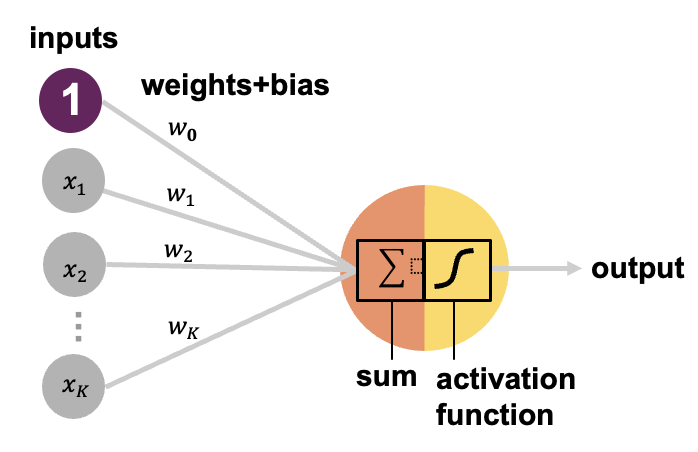
A neural network consists of many connected neurons organized in layers as shown in Figure 8.6. The first layer is reserved for the inputs, and is referred to as input layer and the last output layer contains the outputs. The input nodes simply pass the information from the data (provided by an input data representation like the numbers indicating the pixel intensities for images) on to the subsequent layer. The layers in-between are refferred to as hidden layers and the number of hidden layers defines the depth of the network. In feed-forward neural networks, subsequent layers are fully conected, i.e. each node from a succeeding layer is connected to all nodes from the preceding layer. There are neither connections between nodes within the same layer nor cycles/loops in the network. The information in this network thus moves in one direction, namely forward, from the input nodes, through nodes in the hidden layer, toward the output nodes. The model parameters of a neural network comprise the weights and biases of all neurons in the network (number of edges/connections).
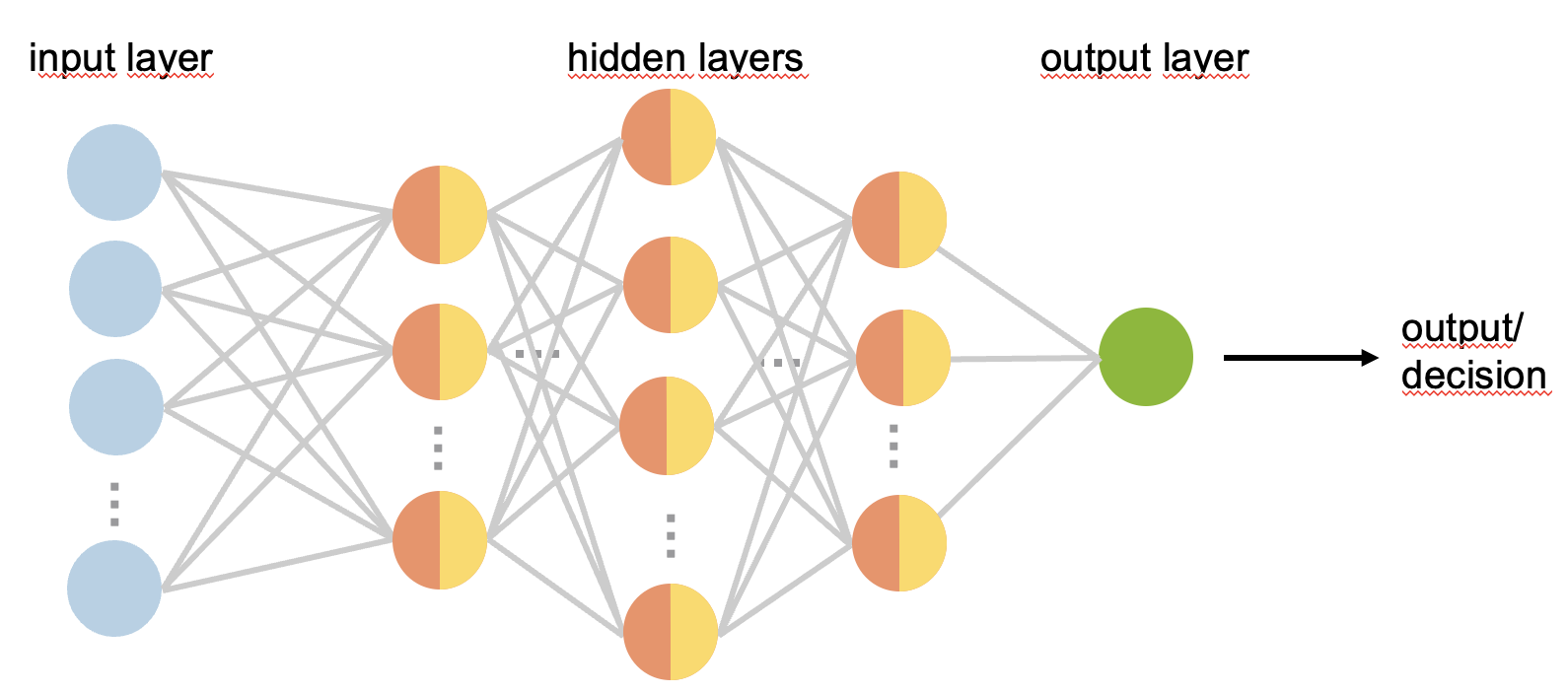
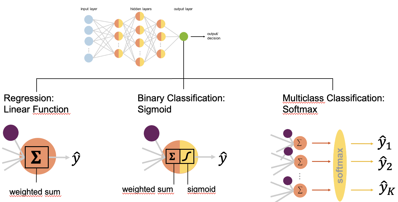
The structure of the output layer depends on the task. For regression tasks (e.g. predict the selling price of a house), the output is a single node corresponding to the prediction computed as a weighted sum of the inputs received from the previous layer (last hidden layer). The output layer has a linear activation function. For a binary classification problem, the output is again a single node computed by applying the logistic (sigmoid) function to the linear combination of its inputs. The outputs are then in the \((0,1)\) interval and can be interpreted as probability or confidence of one of the two class (this is then referred to as the target or positive class). The probability of the other class is 1 minus the predicted probability of the target class. As in logistic regression, a class label is then assigned by using a threshold (e.g. default threshold value is 0.5). When addressing a multiclass classification problem, the number of nodes in the output layer equals the number of different classes. Each node is computed as a linear combination of the inputs received from the previous layer (last hidden layer) and a softmax function to obtain the class probabilities for all different classes for a target input example. The predicted class label corresponds to the class with the highest probability. Such layer is referred to as softmax layer. This is depicted in Figure 8.7.
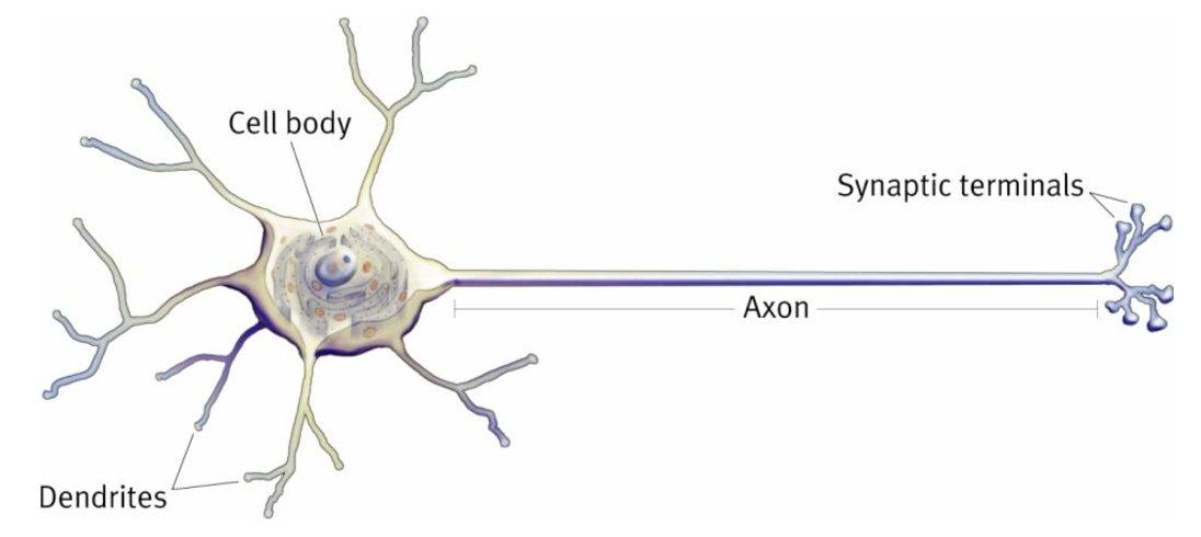
The design of the neuron and the neural network was motivated by the biological neuron shown in Figure 8.8. Biological neurons consist of dendrites, cell body, and axon with synaptic terminals. A neuron is connected to other neurons with thousands of synapses. Once inputs received by the dendrites exceed a certain level a neuron discharges an electrical pulse from the cell body down to the end of the exon and this way transfers signals to other neurons.
8.3 Activation Functions
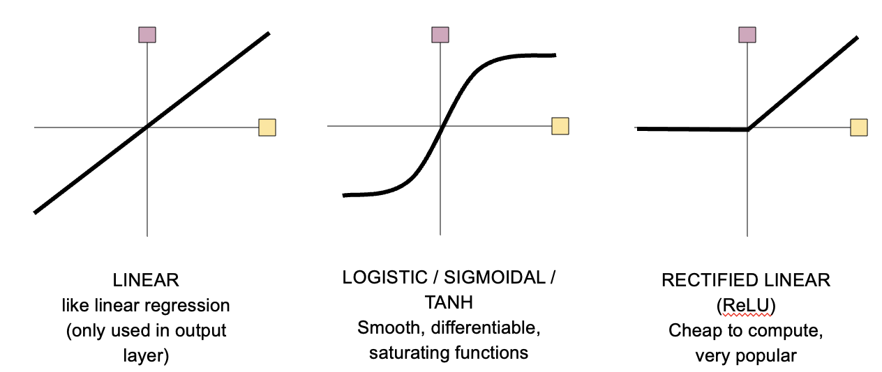
The activation function is the function applied in each neuron to the linear combination of its inputs. The activation function in all layers but the last one for regression (the output layer) is typically a non-linear function. The most commonly used activation functions are given in Figure 8.9. A detailed listing of activation functions can be found under activation functions.
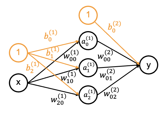
Note that a neural network is still just a function that maps an input to output. This mapping for a small network with a single input, single output and one hidden layer with three neurons depicted in Figure 8.10 is given by: \[ \hat{y}=f[x, \mathbf{\phi}]=b_{0}^{(2)}+w_{00}^{(2)} \zeta[b_{0}^{(1)} + w_{00}^{(1)}x] + w_{01}^{(2)} \zeta[b_{1}^{(1)}+w_{10}^{(1)}x] + w_{02}^{(2)} \zeta[b_{2}^{(1)}+w_{20}^{(1)}x] \] where \(\mathbf{\phi}=\{b_{0}^{(1)}, b_{1}^{(1)}, b_{2}^{(1)}, w_{00}^{(1)}, w_{10}^{(1)}, w_{20}^{(1)}, b_{0}^{(2)}, w_{00}^{(2)}, w_{01}^{(2)}, w_{02}^{(2)}\}\) are the model parameters, \(\zeta\) is the activation function and \(a_{i}^{(1)}=\zeta[b_{i}^{(1)}+w_{i1}^{(1)}x]\) for \(i \in \{0,1,2\}\).
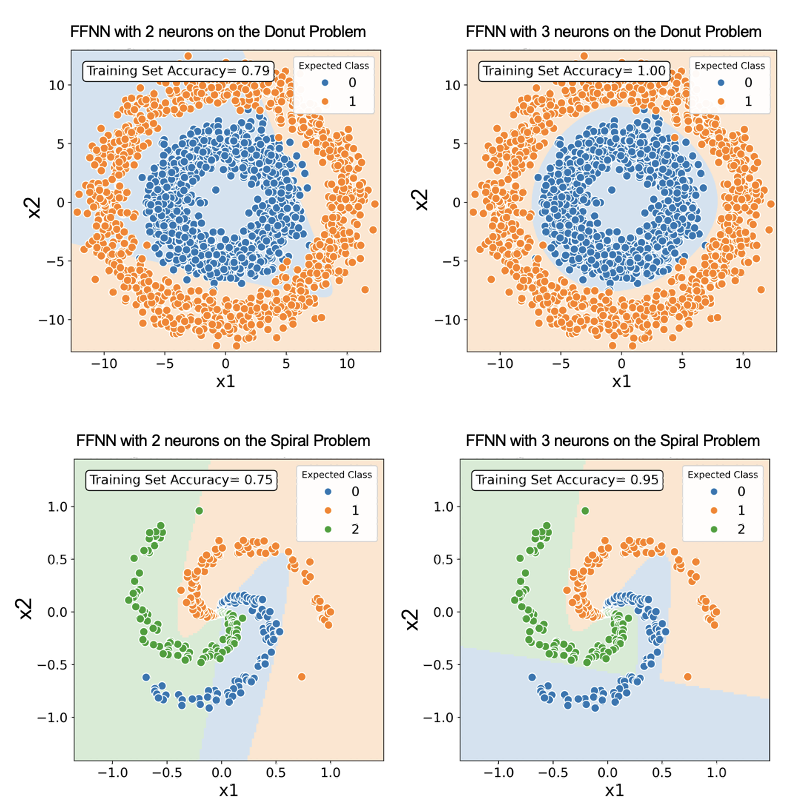
If all activation functions in a neural network were linear then we would end up with a linear model (linear regression for a network addressing a regression problem). A neural network model is non-linear only when it has least one hidden layer with non-linear activation function. Examples of non-linear decision bounderies obtained by neural networks are depicted in Figure 8.11.
8.4 Universality Theorem
Universality theorem (Hornik, 1991): A neural network with one hidden layer using nonlinear activation function can approximate any given continuous function to any desired level of accuracy given enough hidden units.
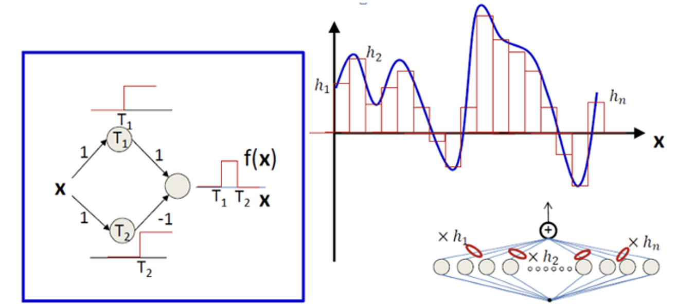
Proof sketch for one-dimensional input: A neural network with one input, one output, and one hidden layer with two neurons and sigmoid activation function, can approximate a step function. Recall that having very large weight in the sigmoid function makes the function very steep (left-most figure in Figure 8.12 showing output of top neuron). The bias (offset) weight moves the step from the origin to the left or right (middle figure in Figure 8.12 showing output of top neuron). By having an additional neuron with a negative weight to the output layer and same magnitude as the top neuron, we get a bar with height equal to the magnitude of the weight (right-most figure in Figure 8.12 showing the output for the bottom neuron).

We can cut an arbitrary continuous function \(f\) in many tiny pieces, then use two neurons to model each piece by a step function. The smaller the pieces, the more precise is the approximation. This is illustrated here:
[Optional] You find more details at universality theorem visual proof.
8.5 The Cost Function
In order to train a neural network model we need to specify a cost function that quantifies how far our predictions are from the actual output values suitable for the target task. If we are addressing a regression task (e.g. predict the selling price of a house), then a suitable cost function is the mean squared error defined as: \[MSE = \frac{1}{M}\sum_{m=1}^{M}(y^{(m)}-\hat{y}^{(m)})^2\] For a binary classification task the logistic cost function is typically used: \[L_{logistic}=-\sum_{m=1}^{M}[y^{(m)}log(\hat{y}^{(m)})+(1-y^{(m)})log(1-\hat{y}^{(m)})]\] For multiclass (multinomial) classification the cross-entropy cost function is often used in practice, specified by: \[L_{CE}=-\sum_{m=1}^{M}\sum_{k=1}^{K}y^{(m)}_k log(\hat{y}^{(m)}_k)=-\sum_{m=1}^{M}log\frac{\exp{(\mathbf{w}^T_{c_m}\mathbf{x}^{(m)})}}{\sum_{k=1}^{K}\exp{(\mathbf{w}^T_k\mathbf{x}^{(m)})}}\] where \(c_m\) the correct class (label) for the \(m\)-th sample.
8.6 Training Neural Networks
Training a neural network translates to finding the model parameters that minimize the cost function. In practice the minimization is computed using gradient descent:
- Initialize all network parameters (the weights) randomly
- Compute the gradient of the cost function with respect to each of the model parameters
- Adjust the model parameters by a small step \(\alpha\) (the learning rate) in the opposite direction of the gradient: \[\mathbf{w} = \mathbf{w} - \alpha \frac{\partial L}{\partial \mathbf{w}}\]
The process of training neural networks with gradient descent referred to as backpropagation is shown in Figure 8.14. After specifying the network architecture (e.g. number of hidden layers, number of neurons per layer, activation function, loss/cost function, learning rate), the network weights (model parameters) are initialized with some random numbers. Then, using these model parameters each training sample is processed through the network in the feed forward pass to compute the output. Remember a network specifies a function that for a given input computes the output. Once we have computed the output we can obtain the loss of the sample that quantifies how good the prediction is compared to the actual target value for the training sample considered. In order to apply gradient descent, one needs to compute the gradient of the loss with respect to all model parameters, and these are many which also means that many computations are needed. However, since partial derivatives in earlier layers are composed of contributions from partial derivatives of later layers, when starting from the parameters in the last layer going backward towards the first layer, one can reuse computations and make the process more efficient. This is why this is called backpropagation. The model parameters (weights) are then updated by a small step in the opposite direction of their respective gradients. The process is then repeated for the next training sample using now the updated model parameters.
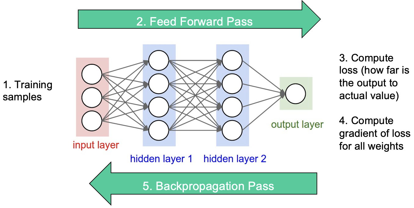
In practice neural networks are trained with mini-batch gradient descent using algorithms with adaptive learning rate (e.g. Adam, AdaGrad, RMSprop). The batch size is the number of training samples in a batch and completing the forward and backpropagation pass for all samples in a batch marks an iteration. An epoch is completed when we have passed through the complete training set, i.e. the forward and backpropagation pass are completed for all training samples (batches).
Note that the loss function for neural networks is not convex as for linear regression. Therefore, there is no guarantee that gradient descent finds the global minimum of the cost function and different parameter initializations might lead to different optimal parameter values. However, the prediction quality of the results obtained by gradient-descent-based approaches for cost minimization is very good. This is the reason why they are the methods of choice in practice.
Next we delve into backpropagation.
8.7 Backpropagation
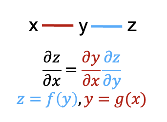
Backpropagation uses the chain rule for partial derivatives depicted in Figure 8.15 that specifies the computation of the partial derivative of a function composition \(z=f(g(x))\) with respect to \(x\) that quantifies how \(z\) changes with very small changes of \(x\).
You can find the derivatives of common function here.
The video 3Blue1Brown Intuitive Walkthrough of Backpropagation gives a very nice intuitive overview of training neural networks with backpropagation, and the video 3Blue1Brown Backpropagation Calculus provides the details of the derivation. Take some time to watch these videos.
In the following we will provide the details of the derivation for a simple chain neural network where each layer has a single neuron shown in Figure 8.16. The bias terms are explicitly depicted in violet as in Figure 8.4. We will follow the notation of the video.

The training data consists of just one sample with (input, output)-value: (\(x\),\(y\)). The neural networks has \(L\) layers, each with a single neuron. The node of the input (zeroth) layer \(a^{(0)}\) is not a neuron and just passes the input value \(x\) into the network: \(a^{(0)}=x\). The neuron of the last layer produces the output of the neural network \(\hat{y}=a^{(L)}\).
Each neuron of layers \({l=1,...,L}\) calculates the linear function (the preactivation): \[
z^{(L)} = w^{(L)}\cdot a^{(L-1)} + b^{(L)}
\]
and produces the output with an activation function \(\zeta\). This could for example be the sigmoid activation function \(\zeta(z)\): \[ a^{(L)}=\zeta(z^{(L)}) = \frac{1}{1+e^{-z^{(L)}}} = \left(1+e^{-z^{(L)}}\right)^{-1} \]
The cost function \(C\) is a function of the training data (\(x\),\(y\)) and the model parameters that quantifies how well the predictions match the observed outputs: \[ C:C\left(x,y;w^{(1)},b^{(1)},w^{(2)},b^{(2)},...,w^{(L)},b^{(L)}\right) \] For simplicity, we select the squared error cost: \[ C = \left(y-a^{(L)}\right)^2 \] Now we need to quantify how changes in the model parameters affect the cost function such that we can make the adjustments of the model paramaters that lead to the most efficient decrease in the cost function. This is reflected in the partial derivatives of the cost function with respect to all model parameters. In the following we will explain this derivation step by step.
We start from the last layer \(L\). In order to compute the partial derivative of the cost function with respect to \(w^{(L)}\) we first draw the computation graph that illustrates the functional dependencies needed to compute \(C\) up to \(w^{(L)}\):
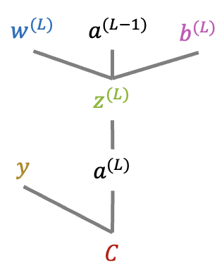
Having this we can easily apply the chain rule: \[ \frac{\partial C}{\partial w^{(L)}} = \frac{\partial C}{\partial a^{(L)}} \cdot \frac{\partial a^{(L)}}{\partial z^{(L)}} \cdot \frac{\partial z^{(L)}}{\partial w^{(L)}} \] Next we can derive the expressions for the three partial derivatives above. The first one is given by: \[ \frac{\partial C}{\partial a^{(L)}} = -2\left(y-a^{(L)}\right) = 2\left(a^{(L)} - y\right) \] This needs to be changed accordingly if one uses another loss function (e.g. cross entropy). The next factor is the derivative of the activation function with respect to its argument \(z\), i.e. \(\frac{\partial a^{(L)}}{\partial z^{(L)}} = \zeta'(z^{(L)})\). For the sigmoid activation function it simplifies as follows: \[ \begin{split} \frac{\partial a^{(L)}}{\partial z^{(L)}} &= \frac{\partial }{\partial z^{(L)}} \left(1+e^{-z^{(L)}}\right)^{-1} = (-1) e^{-z^{(L)}} (-1) \left(1+e^{-z^{(L)}}\right)^{-2} = \frac{e^{-z^{(L)}}}{(1+e^{-z^{(L)}})^2} \\ &=\frac{1}{1+e^{-z^{(L)}}} \cdot \frac{e^{-z^{(L)}} + 1 - 1}{1+e^{-z^{(L)}}} =\frac{1}{1+e^{-z^{(L)}}} \left( \frac{1+e^{-z^{(L)}}}{1+e^{-z^{(L)}}} - \frac{1}{1+e^{-z^{(L)}}} \right) \\ &=\frac{1}{1+e^{-z^{(L)}}} \left( 1- \frac{1}{1+e^{-z^{(L)}}}\right) = \zeta(z^{(L)}) \left(1 - \zeta(z^{(L)}) \right) \end{split} \] Note that in case of a different activation function (e.g. \(\tanh\) or ReLU) this needs to be replaced by the appropriate partial derivative.
The partial derivative of the linear function \(z\) with respect to the weight \(w^{(L)}\): \[ \frac{\partial z^{(L)}}{\partial w^{(L)}} = a^{(L-1)} \]
Now that we have derived all three factors we obtain: \[ \frac{\partial C}{\partial w^{(L)}} = 2\left(a^{(L)} - y\right) \cdot \zeta'(z^{(L)}) \cdot a^{(L-1)} \] and using the sigmoid activation function: \[ \frac{\partial C}{\partial w^{(L)}} = \underbrace{2\left(a^{(L)} - y\right)}_{\frac{\partial C}{\partial{a^{(L)}}}} \cdot \underbrace{\zeta(z^{(L)}) \left(1 - \zeta(z^{(L)}) \right)}_{\frac{\partial a^{(L)}}{\partial z^{(L)}}} \cdot \underbrace{a^{(L-1)}}_{\frac{\partial z^{(L)}}{\partial w^{(L)}}} \]
Next we will derive the partial derivative of the cost function with respect to the bias term of the output layer using the sigmoid activation function. The derivation is done the same way as before and the factors marked in blue are those that can be reused from previously: \[ \frac{\partial C}{\partial b^{(L)}} = {\color{blue}\frac{\partial C}{\partial a^{(L)}} } \cdot {\color{blue}\frac{\partial a^{(L)}}{\partial z^{(L)}} } \cdot \frac{\partial z^{(L)}}{\partial b^{(L)}} \] The third factor in the multiplication is equal to one: \[ \frac{\partial z^{(L)}}{\partial b^{(L)}} = \frac{\partial }{\partial b^{(L)}} \left( w^{(L)}\cdot a^{(L-1)} + b^{(L)} \right) = 1 \] Inserting \(\frac{\partial z^{(L)}}{\partial b^{(L)}}\) and marking all factors we can reuse from \(\frac{\partial C}{\partial w^{(L)}}\) in blue we obtain: \[ \frac{\partial C}{\partial b^{(L)}} = {\color{blue} 2\left(a^{(L)} - y\right) \cdot \zeta(z^{(L)}) \left(1 - \zeta(z^{(L)}) \right) } \cdot 1 \]
In the following we compute the partial derivative of the cost \(C\) with respect to the model parameters \(w^{(L-1)}\) and \(b^{(L-1)}\) of layer \(L-1\). The computation graph is:
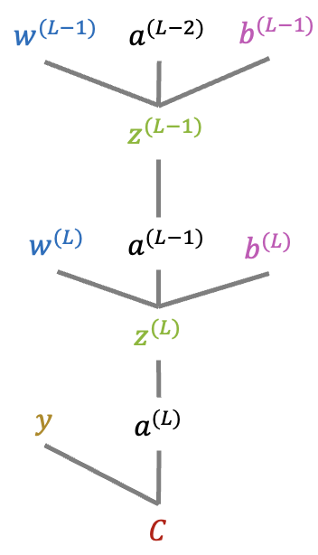
The terms marked in blue can be reused from the computations of the previous layer \(L\): \[ \frac{\partial C}{\partial w^{(L-1)}} = {\color{blue} \frac{\partial C}{\partial a^{(L)}} } \cdot {\color{blue} \frac{\partial a^{(L)}}{\partial z^{(L)}} } \cdot \frac{\partial z^{(L)}}{\partial a^{(L-1)}} \cdot \frac{\partial a^{(L-1)}}{\partial z^{(L-1)}} \cdot \frac{\partial z^{(L-1)}}{\partial w^{(L-1)}} \] The remaining terms (in black) need to be derived:
\[ \frac{\partial z^{(L)}}{\partial a^{(L-1)}} = w^{(L)} \]
\[ \frac{\partial a^{(L-1)}}{\partial z^{(L-1)}} = \zeta\left(z^{(L-1)}\right) \left(1 - \zeta\left(z^{(L-1)}\right) \right) \]
\[ \frac{\partial z^{(L-1)}}{\partial w^{(L-1)}} = a^{(L-2)} \]
Now we can obtain the partial derivatives of the cost function \(C\) with respect to the model parameters \(w^{(L-1)}\): \[ \frac{\partial C}{\partial w^{(L-1)}} = {\color{blue} 2\left(a^{(L)} - y\right) \cdot \zeta(z^{(L)}) \left(1 - \zeta(z^{(L)}) \right) } \cdot w^{(L)} \cdot \zeta\left(z^{(L-1)}\right) \left(1 - \zeta\left(z^{(L-1)}\right) \right) \cdot a^{(L-2)} \] and \(b^{(L-1)}\): \[ \frac{\partial C}{\partial b^{(L-1)}} = {\color{blue} 2\left(a^{(L)} - y\right) \cdot \zeta(z^{(L)}) \left(1 - \zeta(z^{(L)}) \right) \cdot w^{(L)} \cdot \zeta\left(z^{(L-1)}\right) \left(1 - \zeta\left(z^{(L-1)}\right) \right) } \cdot 1 \]
After that we can move on to layer \(L-2\): \[ \frac{\partial C}{\partial w^{(L-2)}} = {\color{blue} \frac{\partial C}{\partial a^{(L)}} } \cdot {\color{blue} \frac{\partial a^{(L)}}{\partial z^{(L)}} \cdot \frac{\partial z^{(L)}}{\partial a^{(L-1)}} \cdot \frac{\partial a^{(L-1)}}{\partial z^{(L-1)}} } \cdot \frac{\partial z^{(L-1)}}{\partial a^{(L-2)}} \cdot \frac{\partial a^{(L-2)}}{\partial z^{(L-2)}} \cdot \frac{\partial z^{(L-2)}}{\partial w^{(L-2)}} \]
\[ \frac{\partial C}{\partial b^{(L-2)}} = {\color{blue} \frac{\partial C}{\partial a^{(L)}} } \cdot {\color{blue} \frac{\partial a^{(L)}}{\partial z^{(L)}} \cdot \frac{\partial z^{(L)}}{\partial a^{(L-1)}} \cdot \frac{\partial a^{(L-1)}}{\partial z^{(L-1)}} \cdot \frac{\partial z^{(L-1)}}{\partial a^{(L-2)}} \cdot \frac{\partial a^{(L-2)}}{\partial z^{(L-2)}} } \cdot \frac{\partial z^{(L-2)}}{\partial b^{(L-2)}} \]
and so on…
The reuse of previous computations (those of later layers of the network) makes backpropagation efficient.
Note that in our simple example our training set had just one sample. When the training set has many samples, the partial derivatives are also averaged among all training samples. This is the case because the cost function is computed as the average over the individual costs for all training samples.
If we have multiple neurons per layer, we will also have multiple paths that influence the computation of the cost function and the partial derivatives of each path needs to be added.
8.8 Vanishing and Exploding Gradient Problems
If a neural network has many hidden layers (as it is the case in deep neural networks), then one ends up with a long chain of multiplications especially when computing the partial derivatives of the early layers. If the partial derivatives are small (in the case of the sigmoid function they are between -1 and 1) then multiplying them will result in exponentially small values. This means that the parameters in early layers will change very slowly which results in a very slow training process. This is referred to as the vanishing gradient problem. If the partial derivatives are large then long chain of multiplications results in very large numbers and this is referred to as the exploding gradient problem. Advanced network architectures address these problems.
8.9 Dealing with Overfitting
Neural networks, known for their flexibility and numerous parameters, are prone to overfitting the training data. To mitigate this, various strategies are employed in practice. We will discuss three commonly used techniques to prevent overfitting in neural networks.
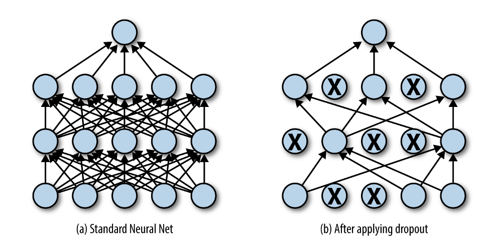
Dropout: This technique illustrated in Figure 8.19 is used to prevent overfitting in neural networks by deactivating a randomly selected proportion of the neurons during training. This means that in each training iteration, a certain percentage of the neurons (along with their connections) are randomly selected and dropped out or ignored. In the next iteration another random subset is deactivated and so on. This randomness forces the network to not rely excessively on any specific set of neurons, promoting a more distributed and robust learning across all neurons. As a result, the network becomes less sensitive to specific weights, leading to a reduction in overfitting. Note that drop out is only applied in the model training process. During inference or testing the full network with all neurons is used with scaled activations to account for the drop out during training. The drop out percentage is a hyperparameter and needs to be selected via model selection using for example a validation set. Typical dropout rates are in the range of 20-50%.
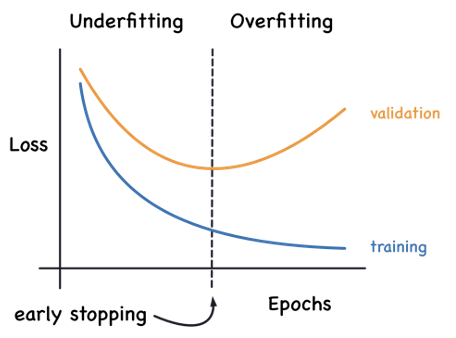
Early Stopping: This is a technique to prevent overfitting in neural networks by terminating the training process before the model has reached the point of overfitting. This is done by performing periodical performance evaluation (e.g. every 5 epochs) of the method on a validation set during model training. If the model’s performance on the validation set starts to worsen (indicating potential overfitting), the training is stopped. The goal is to halt the training process at the point where performance on unseen data is optimal. This is illustrated in Figure 8.20.
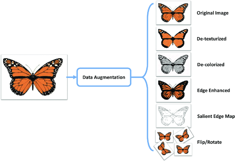
Data Augmentation: This is an approach used to increase the size and diversity of training data without actually collecting or labelling new data. This is achieved by applying various meaningful transformations (adding some random noise) to existing data samples to create altered versions. In the context of images, these transformations can include rotations, scaling, cropping, flipping, adjusting brightness or contrast, decolorizing and so on (Figure 8.21). For text data, meaningful transformations involve synonym replacement (as shown in Figure 8.22) or translation back and forth between different languages. In the context of audio data, an approach to data augmentation involves masking sections of frequency channels and time steps in the mel spectrogram representation as illustrated in Figure 8.23.


8.10 Hyperparameters
Neural networks have many hyperparameters than can affect the quality of their predictive performance. These include, the number of layers, the number of neurons in each layer, the activation function, the optimization algorithm (e.g. Adam, RMSprop, Momentum, …) and its parameters (learning rate), whether to use drop out and the percentage, whether to use early stopping, whether to use data augmentation (types of transformations make sense and how many augmented samples), the batch size, the number of epochs and so on. These are all knobs that can be adjusted and selected using a validation set and analyzing the learning curves obtained.
8.11 Neural Network Topologies
In this section we have focused on the vanilla feedforward neural networks. There are many other network topologies, such as convolutional neural networks, residual networks or transformers, that deliver excellent results on challenging tasks like image classification, speech recognition or question answering. Their development is often motivated by a the characteristics of the input data, a specific application and/or the shortcomings of existing models (vanishing gradients).
8.12 Frameworks
There are several frameworks that offer simple interfaces for building neural network models and automatic differentiation. The most frequently used ones currently are TensorFlow, Keras (build on top of TensorFlow to offer a simpler interface) and PyTorch. HuggingFace is a very useful platform that provides many pre-trained deep learning models and datasets.