10 Clustering
10.1 Unsupervised Learning
In unsupervised learning the training data does not contain any output (target) values: we are only given the input features, e.g. properties of houses such as the size of the house, the number of bedrooms, the size of the plot and so on. The goal is to model the underlying distribution of the data \(\mathbf{X}\) (describe the structure of the data, discover hidden patterns), in order to explain it, to apply the model to new data and obtain practically relevant insights. This brings additional challenges compared to supervised learning:
- The problem statement is much fuzzier
- The evaluation is more difficult without test data including expected output values
A prominant example of unsupervised learning is clustering which is the focus of this chapter.
10.2 What is clustering?
Clustering is the task of grouping a set of objects in such a way that objects in the same group (called a cluster) are more similar (in some sense) to each other than to the objects in the other groups (clusters). Grouping the datapoints can help us to better understand the data and take informed practically-relevant decisions based on that understanding. For instance, if we identify a group of similar cancer patients, we might be able to find a pattern that is related to the origin of their cancer.
10.3 Definition: Clustering
Given a set of \(M\) data points \(X=\{x^{(1)}, x^{(2)}, \ldots, x^{(M)}\}\), where each data point consists of \(n\) features \(x^{(i)} = (x_{1}^{(i)}, \ldots, x_{N}^{(i)}) \in \mathbb{R}^{N}\), and a distance measure \(d\), a clustering is a collection of subsets of \(X\) referred to as clusters. The clusters are created with the goal that samples in the same cluster are similar, i.e. have a small distance according to the distance measure \(d\), whereas samples belonging in different clusters have a large distance \(d\). The goal of a clustering task is to separate the data into \(K\) clusters.
10.4 Example
Assume we have a training set with \(M=16\) data points where each of them consists of two measurements (\(N=2\)): height and weight, depicted in the left image in Figure 10.1. Then we might partition the data in two clusters (as shown in the plot in the middle image in Figure 10.1), or into 5 clusters (as shown in the plot in the right image in Figure 10.1).

10.5 Types of Clustering
There are two types of clustering:
- Hard clustering: Each data point is assigned a unique cluster (belongs to one cluster);
- Soft clustering: Each data point \(m\) is assigned a probability \(p_{km}\) that it belongs to cluster \(k\) for \(k=1:K\) (\(K\) being the total number of clusters) such that \(\sum_{k}p_{km}=1\).
In the following we will focus on two methods for hard clustering, K-Means and DBSCAN.
10.6 The K-Means Algorithm
One of the most prominent clustering algorithms is the K-Means algorithm. The main idea is shown in the following video.
The following pseudo-code depicts the basic principles of K-Means:
Input:
- \(X = \{x^{(1)}, \ldots, x^{(M)}\}\) set of \(M\) data points
- The number of clusters \(K\)
Output:
- A set of \(K\) centroids \(\{c_1, \ldots, c_K\}\)
Algorithm
Specify the number of clusters \(K\) Choose K initial centroids \(c_1, \ldots, c_K\)
REPEAT
Compute closest centroid \(c_k\) for each data point and “assign” data point to that centroid
FOR EACH centroid \(c_k\)
- \(A_k\) = set of data points currently assigned to \(c_k\)
- \(m_k = \frac{1}{|A_k|}\sum_{x^{(m)} \in A_k} x^{(m)}\) (mean of all data points in \(A_k\))
- \(c_k = m_k\)
END FOR
UNTIL stop-criterion is met
RETURN \(c_1, \ldots, c_K\) as the centroids of the \(K\) clusters
In the pseudoalgorithm above each loop consisting of assigning data points to cluster centroids and recomputing the centroids is referred to as iteration. Note that the K-Means algorithm tends to find spherical clusters.
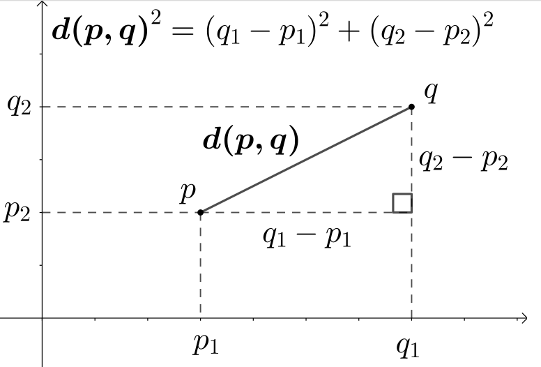
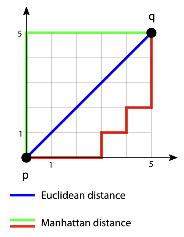
Distance measure: For the distance between two data points the Euclidean distance (L2-norm) is used defined as \(d(p,q)=\sqrt{\sum_{i = 1}^{N} (q_{i} - p_{i})^{2}}\) for two \(N\)-dimensional points \(p\) and \(q\). An example for \(N=2\) (two-dimensional points) is given in Figure 10.2.
10.7 Selection of initial centroids
There are three simple ways to select the initial centroids at the beginning of the algorithm:
- Random points randomly selects \(K\) points in \(\mathbb{R}^N\);
- The Forgy method randomly chooses K observations from the dataset and uses these as the initial means;
- The Random Partition method first randomly assigns a cluster to each observation and then proceeds to the update step, thus computing the initial mean to be the centroid of the cluster’s randomly assigned points.
A more sophisticated approach to selecting the initial cluster centers is K-means++:
- Randomly select the first centroid from the data points
- For each data point compute its distance from the nearest, previously chosen centroid (the minimum distance from all centroids)
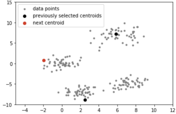
- Select the next centroid from the data points such that the probability of choosing a point as centroid is directly proportional to its squared distance from the nearest, previously chosen centroid. (i.e. the point having maximum distance from the nearest centroid is most likely to be selected next as a centroid)
- Repeat steps 2 and 3 until K centroids have been sampled.
An example of one centroid selection (the one depicted in red color) with K-means++ is given in Figure 10.3.
10.8 Stop-Criterion
There are many potential stopping criteria for the K-Means algorithm. The most obvious one is to stop when the centroids do not change anymore. This also means that the assignment of data points to centroids does not change anymore (it is “stable”), and we can output the result.
However, for large data sets we cannot expect that we will reach such a stable assignment in reasonable time. Instead, we expect that after some time the assignment will only change “slightly”, which we can assess with any of the following criteria:
- Stop when the coordinates of the centroids change only very little from one iteration to the next
- Stop when only very few data points are re-assigned to a different centroid in a new iteration.
Apart from this, we can also use time-boxed criteria:
- Stop after a fixed number of iterations (e.g. after 20-50 iterations)
- Stop after a certain time for the entire computation has elapsed (e.g. after 1 minute).
10.9 Quality of K-Means Clustering
Note that because of the random initialization, the clusters found by K-means can vary from one run to another and different initial centroids might result in very different clusterings. For this reason, we need a way to quantify the quality of a clustering. This is typically done by using the potential function \(\Phi\) which measures the squared distance between each data point and its closest centroid:
Let \(C = \{c_1, \ldots, c_K\}\) denote a set of \(K\) centroids, then \(\Phi(C, X) = \sum_{m = 1}^{M} min_{c \in C} (d(x^{(m)}, c)^{2})\).
In practice, one will run K-Means clustering algorithm several times with different randomly selected initial centroids, and then choose the best clustering that was obtained as quantified by the potential function.
10.10 Choosing the number of clusters K
The K-means clustering method requires that we specify the total number of clusters \(K\). If we know how many clusters we are expecting in the data - e.g. because we want to have a specific number of clusters for subsequent processing, or we have obtained the correct number from domain experts - then we can just select the proper value for \(K\).
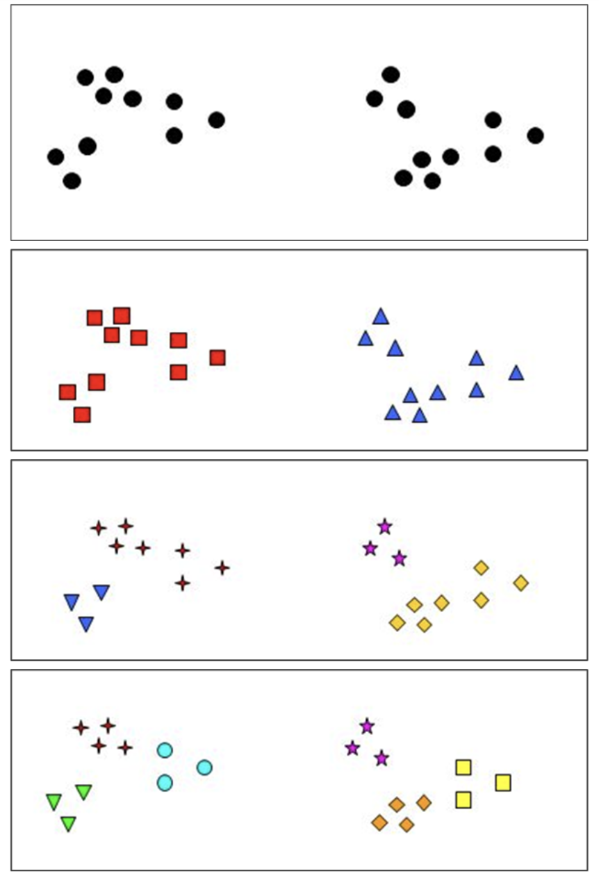
However, in most cases, clustering aims to discover the hidden structure in the data and it is not clear what the correct number of clusters is. In fact, in many cases different values for \(K\) are reasonable. For instance, in the following picture having either \(2\) or \(6\) clusters seems obvious, but also \(4\) clusters might be a reasonable option:
There are different approaches used to determine a good value for \(K\). We will describe two of them, namely, the Elbow Method and the Silhouette Method.
10.11 The Elbow Method
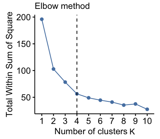
In this method, we run K-Means with different values of \(K\) and plot the value of the potential function \(\Phi\) for each value of \(K\).
Then the value of \(K\) at the point where the slope of the curve significantly decreases (or where the elbow would be if we imagine an arm along the curve) is a good choice for the number of clusters. This is because afterwards the improvements are only marginal.
Applying this approach in the example in Figure 10.5, we would set \(K=4\).
10.12 The Silhouette Method
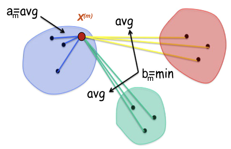
Silhouette Score. Given K clusters computed with a clustering algorithm, given any data point \(x^{(m)}\), let \(a_m\) be the average distance (e.g. Euclidean distance) of \(x^{(m)}\) with all other points in the same cluster. \(a_m\) measures how well the data point \(x^{(m)}\) fits into its own cluster. Let \(b_m\) be the smallest average distance of \(x^{(m)}\) to all points in any other clusters of which \(x^{(m)}\) is not a member. This is illustrated in Figure 10.6. The Silhouette Score \(s_m \in [-1,1]\) is then defined as \(s_m=\frac{b_m-a_m}{max(b_m, a_m)}\). Higher values of the Silhouette Score are indicative of better clustering of the target point: \(s_m\) is close to 1 if point \(x^{(m)}\) is in a tight cluster and far away from other clusters; close to 0 if the target point is on or very close to the boundary between neighboring clusters; and close to -1, if it is in a wrong cluster. The Average Silhouette Score (Width) is computed as the average of the Silhouette Scores of all data points in the training set: \(\frac{1}{M}\sum_{m=1}^{M}s_m\).
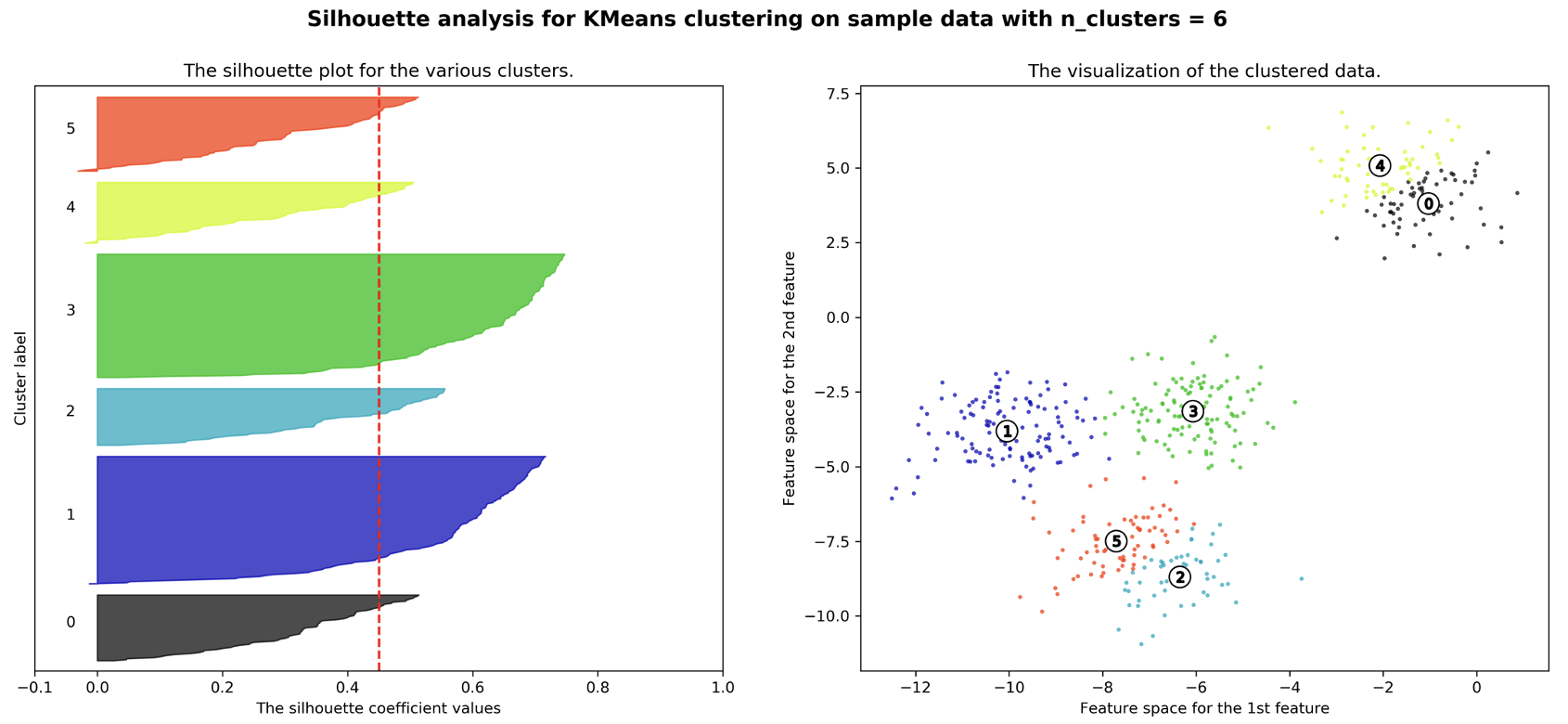
Silhouette Plot: This is the plot of the silhouette scores for all points in the dataset and an example is shown in Figure 10.7. Different colors depict the different clusters. The thickness of the plots for the different colors illustrate the size of the clusters and the red vertical line provides the average silhouette score. In clusters 1, 4 and 5 there are points with negative silhouette scores. In this case trying out 4 clusters might yield more meaningful clustering that combines clusters 4 and 0, and clusters 5 and 2.
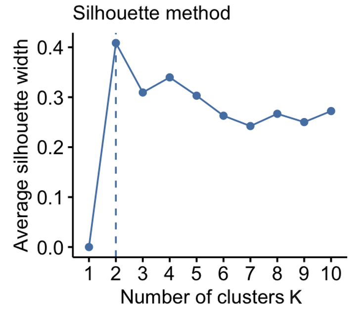
Silhouette Method. The Silhouette Method computes the average Silhouette score for the clustering results obtained by a target algorithm for range of different values of \(K\) and selects the number of clusters \(K\) corresponding to the highest average Silhouette score. In the example in Figure 10.8 we vary \(K\) from 1 to 10 clusters for a K-means clustering algorithm and select \(K=2\) as the optimal value of \(K\) as it results in the highest average Silhouette score.
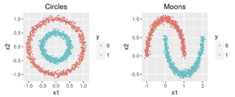
Note that the Silhouette Method might not perform as expected for all data shapes. For the datasets depicted in Figure 10.9 one should rather choose a density-based quality measure such as DBCV (Density Based Clustering Validation) index (optional reading on this one can be found here) or select a different distance measure.
10.13 Runtime Complexity K-Means
Note that solving the K-Means clustering problem - i.e. finding \(K\) centroids that minimize the sum of squared distance to all data points - is NP-hard (see here). In the following, we will analyze the runtime of the K-Means algorithm for the simplest variant, where we select \(K\) random points as initial centroids.
Assume we are given \(M\) data points with \(N\) features. Assume further that K-Means stops after \(L\) iterations. Then the runtime of K-Means is \(\mathcal{O}(LKNM)\).
- In the first step, we randomly select \(K\) initial centroids with \(N\) dimensions each: this step will run in \(\mathcal{O}(KN)\).
- In each of the \(L\) iterations, we compute the distance between each data point and each centroid. The euclidean distance computation takes \(\mathcal{O}(N)\). There are \(M\) data points and \(K\) centroids, thus we need total time \(\mathcal{O}(KNM)\) per iteration.
- There are \(L\) iterations, each taking \(\mathcal{O}(KNM)\), leading to a total runtime of \(\mathcal{O}(LKNM)\).
10.14 DBSCAN
DBSCAN stands for Density-based Spatial Clustering of Applications with Noise and is described in this video. In the following we will summarize it.
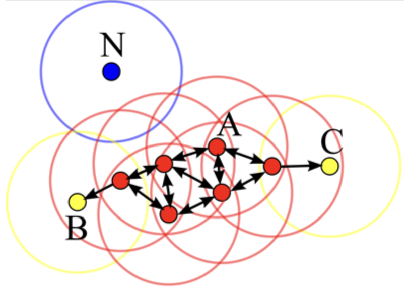
The basic idea of DBSCAN is that clusters form dense regions in the data and are separated by relatively empty areas. Points within a dense region are called core points. DBSCAN identifies points in “densely populated” regions of the feature space in which many data points lie close together.
DBSCAN has two parameters that determine the neighborhood of the points:
- minPts: The minimum number of points (a threshold) clustered together for a region to be considered dense
- \(\epsilon\): A distance measure to define the neighborhood of any point. Point \(p\) is reachable from point \(q\) iff \(distance(p,q) < \epsilon\).
Using these parameters, we can split up the input datapoints into three types of points depicted in Figure 10.10:
- Core point: has at least minPts points within distance \(\epsilon\) from itself (e.g. point A)
- Border point: has at least one core point within distance \(\epsilon\) (e.g. point B, C)
- Noise point: a point that is neither a core nor a border point (e.g. point N).
The DBSCAN Algorithm is described as follows:
- Select an unprocessed point P
- If P is not a Core Point (i.e. there are less than minPts points within range \(\epsilon\)), then classify P as noise and go back to Step 1
- Otherwise, if P is a core point, a new cluster is formed as follows:
- Assign all neighbors of P (i.e. all points within distance \(\epsilon\) from P) to the new cluster
- Repeat previous assignment step for all newly-assigned neighbors that are core points
- Go back to Step 1
- Continue algorithm until all data points have been processed.
The main advantages of DBSCAN is that we do not need to specify the number of clusters \(K\) in advance, it can find clusters with complex, arbitrary shapes and it explicitly identifies outliers (the points tagged as noise points). If, however, there are large differences in the data densities then it does not detect meaningful clusters and OPTICS is an alternative (optional OPTICS).
Runtime DBSCAN: The naive implementation of this algorithm has running time \(O(M^2)\) for \(M\) samples. However, this can be reduced to \(O(M log M)\) with a data structure that allows to retrieve all neighbors of a point \(p\) in time \(O(log M)\). Note that this only works if we assume that there are on average at most \(log M\) neighbors for each point.
[Optional] Further Reading: In-depth description and implementation of DBSCAN can be found here and the original paper is here.
10.15 Distance Metrics
There are other distance metrics, beside the Euclidean one, that can be used to quantify the (dis)similarity among the data points. The following metrics can be used by K-Means and similar algorithms.
Popular metrics are:
- The \(L_1\) metric, known as the Manhattan distance defined as \(d_1(p,q)=\sum_{i}|p_i-q_i|\) and illustrated here:
The \(L_{\inf}\) or the maximum metric defined as \(d_{\inf}(p,q)=\max_{i}\{|p_i-q_i|\}\).
The Cosine similarity defined as \(d_{cos}(p,q)=\frac{\sum_{i=1}^{N}p_iq_i}{\sqrt{\sum_{i=1}^{N}p_{i}^2}\sqrt{\sum_{i=1}^{N}q_{i}^2}}\), quantifies the similarity among two vectors by only accounting for the angle between them and ignoring their lengths. This similarity equals the cosine of the angle between the vectors, and thus, orthogonal vector have a cosine similarity of 1, proportional vectors have a similarity of 1, and opposite vectors have a similarity of -1.