7 Decision Trees
This section is to a large extend based on Chapters 6 and 7 in A. Géron, Hands-On Machine Learning with Scikit-Learn, Keras and Tensorflow, 3rd Edition, O’Reilly Media, Inc. With a public github-repository
Decision trees are versatile machine learning algorithms that can perform both classification and regression tasks. First, the main concepts around visualising, making predictions from and training decision trees are discussed for classification tasks. As a concrete method the CART (Classification and Regression Trees)-Algorithm as implemented in scikit-learn is presented. Then the regularisation of decision trees is discussed.
7.1 Predictions from a Classification Tree
As an introductory example we work with the iris flower dataset. It consists of 3 different types of iris species (Setosa, Versicolor, and Virginica) described by 4 numerical variables: petal length, width and sepal length, width (Figure 7.1).
Figure 7.2 shows a decision tree built on the iris dataset for classification of the species (Setosa, Versicolor and Virginica) based on only two features: petal width and petal length. The classification starts at the root node (depth 0, at the top): this node asks whether the flower’s petal length is smaller than 2.45 cm. If it is, then you move down to the root’s left child node (depth 1, left). By convention, the fraction, for which the split evaluates to True is always on the left side. In this case, it is a leaf node (i.e., it does not have any child nodes), so it does not ask any questions, but outputs the majority class of its samples as a prediction. The most frequent class at the depth-1 left node is Iris setosa, so that is what the decision tree predicts in this case.
For a flower with petal length greater than 2.45 cm you again start at the root but now move down to its right child node (depth 1, right). This is not a leaf node, it is a split node, so it asks another question: is the petal width smaller than 1.75 cm? If it is, then your flower is most likely an Iris versicolor (depth 2, left). If not, it is likely an Iris virginica (depth 2, right).
A node’s samples attribute counts how many training instances it applies to. For example, 100 training instances have a petal length greater than 2.45 cm (depth 1, right), and of those 100, 54 have a petal width smaller than 1.75 cm (depth 2, left). A node’s value attribute tells you how many training instances of each class this node applies to: for example, the bottom-right node applies to 0 Iris setosa, 1 Iris versicolor, and 45 Iris virginica.
Finally, a node’s gini attribute measures its Gini impurity (Equation 7.1): a node is pure (gini=0) if all training instances it applies to belong to the same class. For example, since the depth-1 left node applies only to Iris setosa training samples, it is pure and its Gini impurity is 0. On the other extreme, the root node is a maximally impure node: Each of the three classes is present with the same amount of samples (50), which leads to a Gini impurity equal to \(\approx\) 0.667. See Section 7.2 for the mathematical definition.
Figure 7.3 shows the decision boundaries of the decision tree in Figure 7.2. The vertical boundary represents the decision of the root node (depth 0) at petal length = 2.45 cm. Since the lefthand area is pure (only Iris setosa), it cannot be split any further. However, the righthand area is impure, so the depth-1 right node splits it at petal width = 1.75 cm (horizontal boundary). Since max_depth was set to 2, the decision tree stops right there.
A decision tree can also estimate the probability that a sample belongs to a particular class \(k\). First it traverses the tree to find the leaf node for this sample, and then it returns the ratio of training samples of class \(k\) in this node.
For example, for a flower whose petals are 5 cm long and 1.5 cm wide. The corresponding leaf node is the depth-2 left node in Figure 7.2, so the decision tree outputs the following probabilities: 0% for Iris setosa (0/54), 90.7% for Iris versicolor (49/54), and 9.3% for Iris virginica (5/54). And if you ask it to predict the class, it outputs Iris versicolor (class 1) because it has the highest probability.
7.2 Impurity Measures For Classification
We denote the data at node \(i\) by \(Q_i\) consisting of \(M_i\) samples. If a target is a classification outcome taking on values \(k=1,2,...,K\) for node \(i\), let \[p_{ik} = \frac{1}{M_i}\sum_{y\in Q_i} I(y=k)\]
be the proportion of class \(k\) observations in node \(i\). If \(i\) is a leaf node, \(p_{ik}\) is the predicted probability for this region of the feature space. By default, the DecisionTreeClassifier in scikit-learn uses the Gini impurity measure:
\[G\left(Q_i\right)=1-\sum_{k=1}^K p_{i,k}^2 \tag{7.1}\]
For example, the depth-2 left node in Figure 7.2 has a Gini impurity equal to \(1 – (0/54)2 – (49/54)2 – (5/54)2 \approx 0.168\). If all samples belong to the same class, the Gini impurity becomes zero. The highest Gini impurity for a given number of classes is reached, when each class has the same number of samples.
Another common metric is the entropy:
\[H\left(Q_i\right)=-\sum_{k=1}^K p_{i,k} \log_2 p_{i,k} \tag{7.2}\]
For example, the depth-2 left node in Figure 7.2 has an entropy equal to \(–(49/54) \log_2 (49/54) – (5/54) \log_2 (5/54) \approx 0.445\).
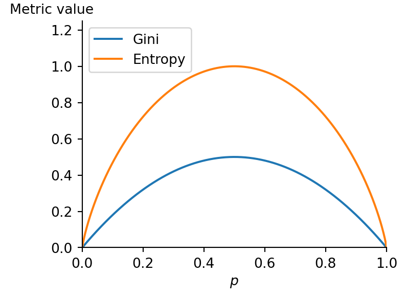
Figure 7.4 shows that Gini impurity and entropy behave very similarly. When all samples belong to the same class, both metrics are zero and both have their maximum at \(p=0.5\), when the classes have the same number of samples.
Most of the time both metrics lead to similar trees. Gini impurity is slightly faster to compute, so it is a good default.
By default, the Scikit-learn DecisionTreeClassifier class uses the Gini impurity measure, but “entropy” can be selected with the criterion hyperparameter.

7.3 Training a Decision Tree for Classification
Scikit-learn uses the Classification and Regression Tree (CART) algorithm to train decision trees. It produces only binary trees, so split nodes always have exactly two children (i.e., questions only have True/False answers).
We denote the data at node \(i\) by \(Q_i\) consisting of \(M_i\) samples. The algorithms starts at depth=0 with a root node \(Q_{i=0}\) where the training set is split into two subsets using a single feature \(n\) and a threshold \(t_{i=0}\) (e.g., petal length \(\leq\) 2.45 cm). Once the CART algorithm has successfully split the training set in two, it splits the subsets using the same logic, then the sub-subsets, and so on, recursively.
How does the algorithm choose the feature \(n\) and threshold \(t_i\) for each split? It searches for the pair (\(n\), \(t_i\)) that produces the purest subsets, weighted by their size.
To achieve this, it sorts all unique values of feature \(n\) among the samples at node \(i\) and calculates the midpoints between adjacent values. Each of those midpoints is evaluated as a threshold \(t_{i}\) in a candidate split \(\theta=(n,t_{i})\). And those candidate splits \(\theta=(n,t_{i})\) partition the samples on the node \(Q_i\) into two subsets: samples whose feature value \(x_n\) is less than or equal to the threshold value \(t_{i}\) (\(Q_i^{\text{left}}(\theta)\)), and those whose feature value \(x_n\) is greater than the threshold value \(t_{i}\) (\(Q_i^{\text{left}}(\theta)\)). Mathematically, we can write this as
\[Q_i^{\text{left}}(\theta) = \{(x,y)| x_n \leq t_i \} \ \text{ and } \ Q_i^{\text{right}}(\theta) = Q_i \setminus Q_i^{\text{left}}(\theta)\]
The quality of a candidate split of node \(i\) is then quantified by a cost function, which is the weighted average of the impurity of the left and right splits:
\[J(Q_i,\theta)=\frac{m^{\text{left}}_i}{m_i}G\left(Q^{\text{left}}_i\left(\theta\right)\right) + \frac{m^{\text{right}}_i}{m_i}G\left(Q^{\text{right}}_i\left(\theta\right)\right) \tag{7.3}\]
By default, the CART algorithm in scikit-learn, uses the Gini impurity metric (Equation 7.1) for classification tasks. However, also the entropy can be used (just replace \(G\left(Q_i\right)\) by \(H\left(Q_i\right)\) in Equation 7.3)
In each split, the \(\theta=(n,t_i)\) that minimise the cost function are selected:
\[\theta^\ast=\text{argmin}_\theta J(Q_i,\theta)\]
The subsets \(Q_i^{\text{left}}(\theta^\ast)\) and \(Q_i^{\text{right}}(\theta^\ast)\) are split recursively until the maximum allowable depth is reached (max_depth hyperparameter in scikit-learn), \(M_i<\min_{\text{samples}}\) or \(M_i=1\).
The CART algorithm is a greedy algorithm: it greedily searches for an optimum split at the top level, then repeats the process at each subsequent level. It does not check whether or not the split will lead to the lowest possible impurity several levels down. A greedy algorithm often produces a solution that is reasonably good but not guaranteed to be optimal. Except for very small datasets such a compromise has to be accepted due to the computational complexity of finding the optimal tree.
In principle, the CART-implementation can handle both numerical and categorical features. However, the scikit-learn implementation does not support categorical features.
The recommended approach of using ordinal encoding converts categorical features to integers which the algorithm will treat as numeric (See Encoding categorical features). If the categorical data is not ordinal, this will lead to splits that are based on a label ordering, which is not reflected in the original data. Using one-hot encoding is in the current implementation the only way allowing arbitrary splits not dependent on the label ordering. But it is computationally more expensive.
7.4 Predictions from a Regression Trees
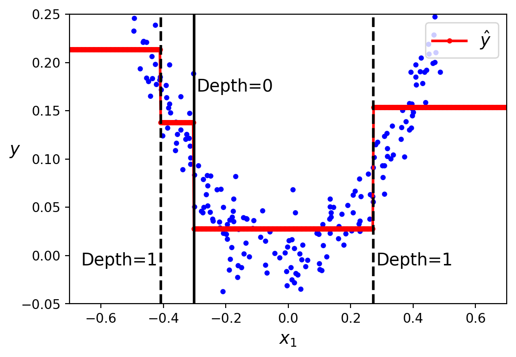
Decision trees can also be used for regression tasks, i.e. the target is a continuous value. In Figure 7.5 we see a tree built to fit the training data in Figure 7.6 (blue dots) up to a maximal depth=2. The main difference to a classification tree is that instead of predicting a class in each node, it predicts a numerical value. For example, to make a prediction for a sample with \(x1 = 0.2\), the root node asks whether \(x1 \leq -0.303\). Since it is not, the algorithm goes to the right child node, which asks whether \(x1 \leq 0.272\). Since it is, the algorithm goes to the left child node. This is a leaf node, and it predicts the value=0.028. This prediction is the average target value of the 110 training samples associated with this leaf node, and it results in a mean squared error equal to 0.001 over these 110 instances.
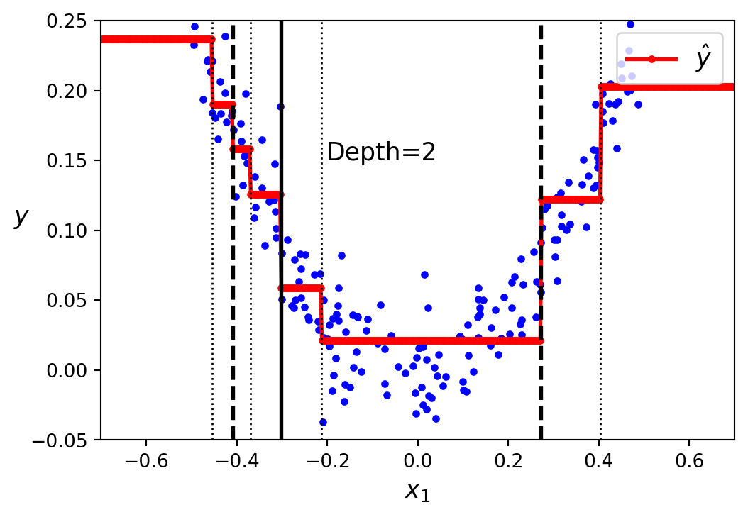
The predictions of the tree in Figure 7.5 are represented in Figure 7.6 as red lines. Each vertical line corresponds to a split node and we end up with the range of the training data target values divided into four regions (4 leaf nodes at depth=2). The predicted value for each region is always the mean value of the training samples in that region, i.e. from that corresponding leaf node. That is, the regression tree approximates the training data as a step function with the steps corresponding to the leaf nodes. With greater depth the model has a greater flexibility to fit the training data with more steps: Figure 7.6 (b) fitted with max_depth=3 compared to Figure 7.6 (a) with max_depth=2.
7.5 Training Regression Trees
To train a decision tree for a regression task with the CART algorithm the same procedure as described for classification in Section 7.3 is applied. However, the impurity metric used to evaluate the candidate splits in Equation 7.3 is different: Instead of the Gini impurity or entropy, the Mean Squared Error (\(MSE\)) is used:
\[MSE(Q_i)=\frac{1}{M_i}\sum_{y\in Q_i} \left(y-\bar{y}_i\right)^2 \tag{7.4}\] with \[\bar{y}_i=\frac{1}{M_i}\sum_{y\in Q_i} y\]
In this case, the predicted value of leaf nodes is set to the learned mean value \(\bar{y}_i\) of the node.
7.6 Regularisation
Decision trees make very few assumptions about the training data (as opposed to, for example, linear models, which assume that the data is linear). If left unconstrained, the tree structure will adapt itself to the training data, fitting it very closely, most likely even overfitting it. Such a model is often called a nonparametric model, not because it does not have any parameters (it often has a lot) but because the number of parameters is not determined prior to training, so the model structure is free to stick closely to the data. In contrast, a parametric model, such as a linear model, has a predetermined number of parameters, so its degree of freedom is limited, reducing the risk of overfitting (but increasing the risk of underfitting).
To avoid overfitting the training data, the decision tree’s freedom needs to be restricted during training similarly as in polynomial regression or SVMs. This is called regularisation. In scikit-learn max_depth and a few other hyperparameters control the stopping conditions to restrict the maximum depth of the decision tree, which will regularise the model and thus reduce the risk of overfitting.
max_depthThe maximum depth of the tree. With the default value
None, nodes are expanded until all leaves are pure or until all leaves contain less than min_samples_split samples.min_samples_splitMinimum number of samples a node must have before it can be split
min_samples_leafMinimum number of samples a leaf node must have to be created
min_weight_fraction_leafsame as min_samples_leaf but expressed as a fraction of the total number of weighted instances
max_leaf_nodesmaximum number of leaf nodes
max_featuressets the number of features that are evaluated for splitting at each node.
Increasing min_* hyperparameters or reducing max_* hyperparameters will regularize the model.
Other algorithms than CART work by first training the decision tree without restrictions, then pruning (deleting) unnecessary nodes.
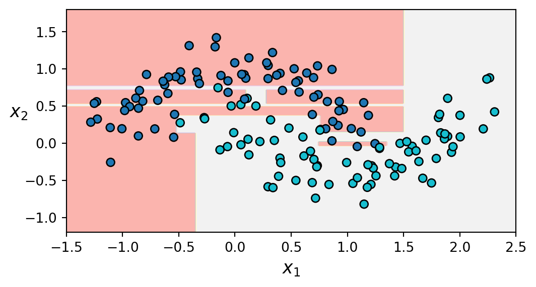
Figure 7.7 shows the effect of the hyperparameter min_samples_leaf on fitting a decision tree classifier on the moons dataset, which is non-linearly separable. A decision tree without regularisation produces the decision boundaries in Figure 7.7 (a), which overfit the data. Another tree with min_samples_leaf=5 leads to a more balanced decision boundary, which generalises better. This can also be verified quantitatively by evaluating both trees on an independent test set.
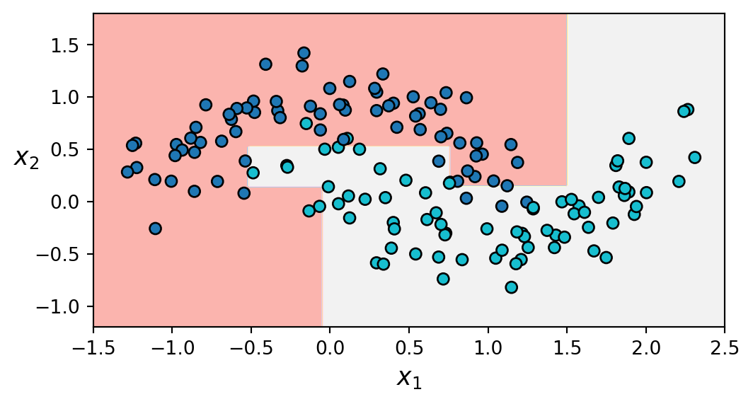
min_samples_leaf=5
Just like for classification tasks, decision trees are prone to overfitting when dealing with regression tasks. Without any regularisation (i.e., using the default hyperparameters in scikit-learn), you get the predictions in Figure 7.8 (a). These predictions are obviously overfitting the training set. Just setting min_samples_leaf=10 results in a much more reasonable model, represented in Figure 7.8 (b).
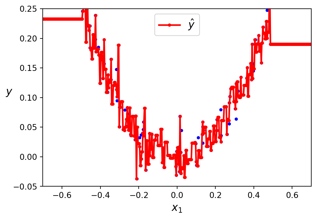
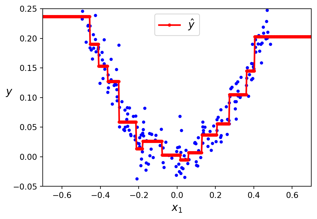
min_samples_leaf=10
7.7 Model Interpretation: White vs. Black Box Algorithms
Decision trees are intuitive, and their decisions are easy to interpret. Such models are often called white box models. In contrast, as you will see, random forests and neural networks are generally considered black box models. They make great predictions, and you can easily check the calculations that they performed to make these predictions; nevertheless, it is usually hard to explain in simple terms why the predictions were made. For example, if a neural network says that a particular person appears in a picture, it is hard to know what contributed to this prediction: Did the model recognize that person’s eyes? Their mouth? Their nose? Their shoes? Or even the couch that they were sitting on? Conversely, decision trees provide nice, simple classification rules that can even be applied manually if need be (e.g., for flower classification). The field of interpretable ML aims at creating ML systems that can explain their decisions in a way humans can understand. This is important in many domains—for example, to ensure the system does not make unfair decisions.
7.8 Random Forests
Random Forests are a type of ensemble methods, that are composed of indvidual decision trees. The principle behind ensemble methods is that aggregating the predictions of a group of different models (an ensemble - see Figure 7.9) often leads to better predictions than from the best individual model alone, provided the individual models are sufficiently diverse, that is independent from one another. This increases the chance that they will make very different types of errors, improving the ensemble’s accuracy.
Generally, the individual trees are trained by the bagging (short for Bootstrap AGGregatING) method. The bootstrap refers to the strategy of generating diversity among the trees: Each tree is trained on a different subset randomly sampled from the complete training set (Figure 7.10). In scikit-learn the size of the subset is controlled with the max_samples parameter (default is the same size as the training set). In the bagging approach this sampling is performed with replacement1. On the other hand, if the sampling is done without replacement it is called pasting. Note that both bagging and pasting allow training instances to be sampled several times across multiple models of the ensemble, but only bagging allows training samples to be sampled several times for the same model.
Once all trees are trained, the ensemble can make a prediction for a new instance by aggregating the predictions of all trees. For regression tasks (RandomForestRegressor) this is done by averaging the predicted values. For classification tasks (RandomForestClassifier in scikit-learn) this is typically done by hard voting or soft voting. Hard voting returns the majority class. The soft voting approach takes into account the individual class probabilities by returning the class with the highest cumulated probability among the individual classifiers, provided they can actually return a probability with their predictions.
Each individual model has a higher bias than if it were trained on the original training set, but aggregation reduces both bias and variance. Generally, the net result is that the ensemble has a similar bias but a lower variance than a single tree trained on the original training set.
The random forest algorithm introduces extra randomness, i.e. diversity, when growing the individual trees: Instead of searching for the very best feature when splitting a node (see Section 7.3), it searches for the best feature among a random subset of features. By default, it samples \(\sqrt{N}\) features (where \(N\) is the total number of features - see the max_features_parameter). This results in greater diversity among the individual trees, which in turn leads to a higher bias along with lower variance, generally yielding a model with better generalisibility.
Out-of-Bag Evaluation: With bagging, some training instances may be sampled several times for any given tree, while others may not be sampled at all. The training instances that are not sampled are called out-of-bag (OOB) samples (Figure 7.11).
These OOB samples can now be used to evaluate a bagging ensemble, without the need for a separate validation set: For each OOB sample generate a prediction from each of the trees in which that sample was OOB. In order to obtain a single prediction for each of those OOB samples, the predicted responses are averaged (if regression is the goal) or aggregated by majority vote (in case of classification). Once a prediction for each OOB sample is generated, an accuracy metric can be calculated.
Imagine picking a card randomly from a deck of cards, writing it down, then placing it back in the deck before picking the next card: the same card could be sampled multiple times. Resampling with replacement is called bootstrapping.↩︎