Code
import numpy as np
import matplotlib.pyplot as plt
def g(z):
    return 1./(1 + np.exp(-z))
x = np.linspace(-10, +10, 100)
plt.plot(x, g(x))
plt.show()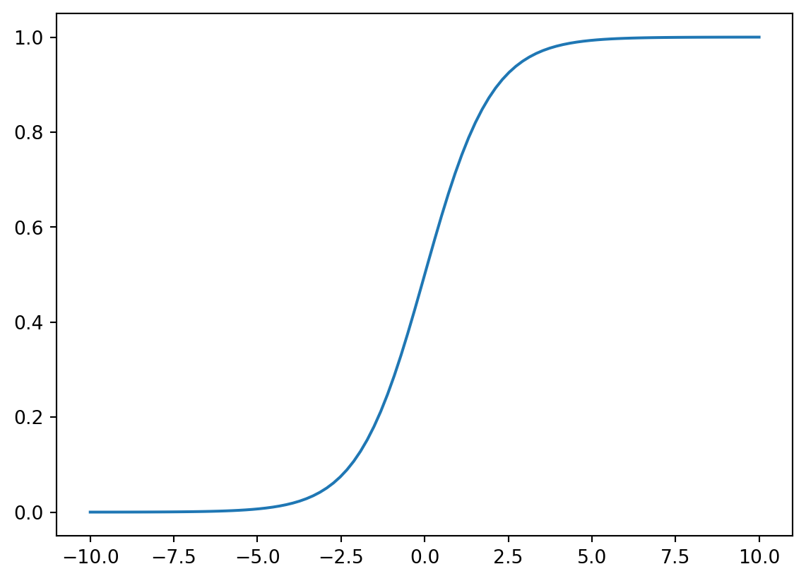
In the previous section we introduced linear regression, which associates an input \(x\) (say, a patient’s cholesterol level in mg/dL) with an output \(y\) (say, their life expectancy in years). Linear regression is useful when (a) \(y\) can be any real number (or an uncountable subset, e.g., all positive real numbers, or all real numbers between 0 and 100), and (b) the goal is for the machine’s estimate \(\hat{y}\) to be as close as possible to the target value \(y\), in the sense of the squared error \((y-\hat{y})^2\). Linear regression is an example of a supervised learning algorithm because, in the training set, the data always appear in pairs: \((x^{(1)}, y^{(1)}), (x^{(2)}, y^{(2)}), \ldots\)
We will now introduce a different supervised learning problem, namely classification. As with regression, the training data comes in pairs. In contrast to regression, the target values \(y\) belong to a finite set. To continue with the medical theme, the set of target values might be \(\{\textrm{flu}, \textrm{cold}, \textrm{covid}\}\), and the machine’s goal is to diagnose a patient who is coughing with a particular disease based on a vector \(x\) of various measurements (body temperature, chest x-ray, mucus sample, etc.). Instead of trying to be “close” to the target value, the goal is to pick the right one as often as possible. There are many classification algorithms, including Decision Trees, Neural Networks, Support Vector Machines, Naive Bayes, Logistic Regression. and many more. Note that we assume here that each \(x\) is associated with exactly one class; hence, in the example above, the patient has exactly one disease (not multiple diseases).
A special kind of classification is binary classification, in which there are only two classes to distinguish. To continue with the medical theme, we might try to use a patient’s cholesterol level \(x\) to predict whether or not a patient will develop heart pain within, say, the next 5 years. In this case, the target value \(y \in \{\textrm{heart pain}, \textrm{no heart pain}\}\). In binary classification, we typically call one class “positive” and the other class “negative” – how you name these is up to you. For instance, “heart pain” might be called “positive”, and “no heart pain” might be called “negative”. However, it could also be the other way round.
How might we tackle binary classification given the machinery we’ve already seen? Naively, we could try using linear regression: Let the value 1 represent “heart pain” and value 0 represent “no heart pain”. We can thus collect a set of training data – in this case, the cholesterol levels \(x^{(1)}, \ldots, x^{(M)}\) of \(M\) patients and the associated outcomes \(y^{(1)}, \ldots, y^{(M)} \in \{ 0,1 \}\). We then train a linear regressor \(h_\theta\), with parameter vector \(\boldsymbol{\theta}\), such that the mean squared error (over all \(M\) training examples) is minimized. While this approach might sound reasonable, it has a problem: The estimate \(\hat{y}\) can be any real number; it is not constrained to be in the set \(\{0,1\}\). This is actually easy to fix. Here’s one approach: after training the linear regressor and determining the optimal \(\boldsymbol{\theta}\), we could transform the “raw” \(\hat{y}\) and force it into the set \(\{0,1\}\) by comparing it to a threshold, say 0.5: if \(h_{\theta}(x) > 0.5\), then we simply declare that \(\hat{y}=1\) (heart pain). In other words, we let \[ h_\theta(x) = \left\{ \begin{array}{cc}1 & \textrm{if}\ \theta_0 + \theta_1 x > 0.5 \\ 0 & \textrm{if}\ \theta_0 + \theta_1 x \leq 0.5 \end{array}\right. \tag{5.1}\] For example, if \(\theta_0=-100\) and \(\theta_1=0.6\), then the hypothesis \(h_{\theta}\) looks as follows:
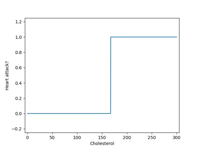
As you can see, this is a “step” function that changes abruptly from 0 to 1 depending on the input \(x\). There are two problems: (1) It throws away potentially useful information about how confident the machine was about its guess for the heart disease. (2) It is a non-differentiable function, which makes it hard to optimize.
To resolve this, we can replace the “hard” (binary) step function with a “soft” (real-valued) step function. In particular, we will use the logistic sigmoid given by the function \[ g(z) = \frac{1}{1 + e^{-z}} \] that is rendered below.
import numpy as np
import matplotlib.pyplot as plt
def g(z):
return 1./(1 + np.exp(-z))
x = np.linspace(-10, +10, 100)
plt.plot(x, g(x))
plt.show()
As you can see, this sigmoid function is “s”-shaped, monotonic (it grows larger from left to right), differentiable, and bounded between 0 and 1. (The function approaches 0 to the left and approaches 1 to the right.) It is the key element of the logistic regression algorithm described in the next section.
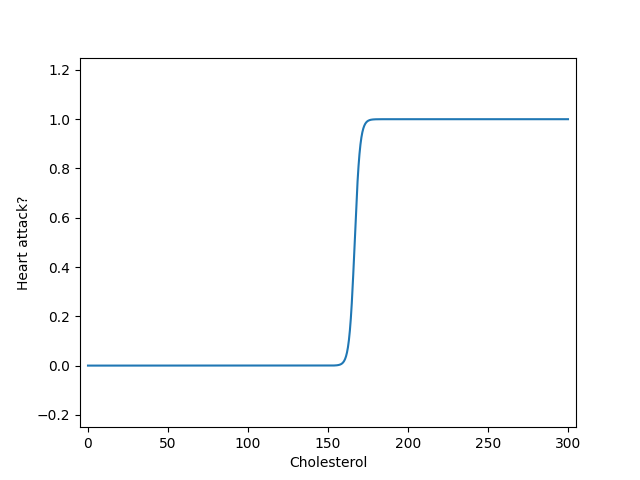
Using the logistic sigmoid \(g\) solves both of the issues of the “hard” step function described above. In particular, we can replace the hard step in Equation 5.1 with the soft step given by \(g\) to yield:
\[ h_\theta(x) = g(\theta_0 + \theta_1 x) \tag{5.2}\]
This results in the following graph:
One of the simplest (and oldest) algorithms for binary classification is logistic regression. (You might be immediately wondering: “why is it called logistic regression if it’s meant for classification?” The answer is likely because, mathematically, it is highly related to linear regression. Try not to let the name confuse you!)
Like linear regression, a logistic regression model has a parameter vector \(\boldsymbol{\theta}\). Once it is trained (and we will describe how training works momentarily), you can apply it to a (unidimensional) input \(x\) as follows: \[\hat{y} = h_\theta(x) = g(\theta_0+ \theta_1 x) = \frac{1}{1 + e^{-(\theta_0 + \theta_1 x)}}\] In other words, you apply it to data \(x\) in the exact same way as linear regression, except that there is one extra step of passing \(\theta_0 + \theta_1 x\) to the sigmoid \(g\).
There is also a straightforward multidimensional generalization: If \(\boldsymbol{x}\) is a vector of numbers, then \[\hat{y} = h_{\boldsymbol{\theta(x)}} = g({\boldsymbol{\theta}}^T \boldsymbol{x}) = \frac{1}{1 + e^{-{\boldsymbol{\theta}}^T \boldsymbol{x}}}\] where \(\boldsymbol{\theta}^T \boldsymbol{x} = \theta_0 x_0 + \theta_1 x_1 + ... + \theta_n x_n\). Here, as in the multivariate linear regression, \(\boldsymbol{x}\) is a vector consisting of \(x_0, x_1, x_2, ...\) and \(x_0=1\), which enables the vector representation of the parameters \(\boldsymbol{\theta}\). In other words, to compute the prediction \(\hat{y}\) for an input \(\boldsymbol{x}\), we must:As you can observe from the s-shaped function \(g\) in Figure 5.2, the output of a logistic regression machine is always between 0 and 1 (and it never quite touches either of these extremes). For a binary classification problem, this is already convenient because you never have to deal with estimates \(\hat{y}\) that are bigger than 1 or smaller than 0. Moreover, the particular value \(\hat{y}\) that you obtain also gives you a sense of how confident the machine is about its judgment. Suppose we apply logistic regression to classify whether a given face image \(\boldsymbol{x}\) (represented as a vector of pixels) is smiling or not. If image \(x\) was very clearly a smile, then \(\hat{y}\) might be very high (say, 0.95). If, on the other hand, the machine thinks the face is a smile but is not very confident, then its output might only be, say, 0.6. If the machine thinks the face is a non-smile but is also not confident, then the output might be something like 0.35; and so on. Of course, how high or low \(\hat{y}\) has to be to be considered “confident” is up to the user, but in most scenarios \(\hat{y}>0.95\) or \(\hat{y}<0.05\) would be considered “confident” whereas \(0.4 < \hat{y} < 0.6\) would be considered “not confident”.
In some settings, you may not care about the confidence value and just want a binary prediction; in this case, you can just threshold \(h_{\boldsymbol{\theta}(\boldsymbol{x})}\) using, say, a threshold of 0.5. In other settings, the probability \(\hat{y} \in (0,1)\) may be more meaningful or useful. Besides giving a sense of the confidence in its prediction, logistic regression also has the advantage over linear regression (when used for classification) that it is more robust to outliers (see Section 5.8).
Note that the parameter vector \(\boldsymbol{\theta}\) – which we optimize based on the training data – determines both the location and the steepness of the soft step function provided by \(g\). Continuing with the heart pain predictor above, if we change \(\theta_0=-50\) and \(\theta_1=0.2\), then we get the following hypothesis function: 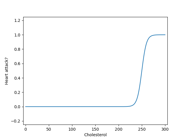
As you can see, the step has moved to the right, and it is slightly less steep than before (since \(\theta_1\) is smaller).
Logistic regression is used for binary classification tasks where the outcome is one of two possible classes. This can be interpreted as predicting the probability that a given input belongs to a certain class (the probability that we get an output that belongs to class 1, given the input data \(x\) (where the output is \(y=0\)) is written \(P(y=0\ |\ x)\) and the probability to get an output in class 2, given the input data \(x\) (where the output is \(y=1\)) is written as \(P(y=1\ |\ x)\)). If the output (probability) is close to 1, then it is one of the classes, and if the output (probability) is close to 0, then it is the other class.
In contrast to linear regression, there is no “normal equation” to find the optimal parameter \(\theta\) in closed form. (Note, that from here on we omit the bold notation for vectors, as the dimensionality is not important, and we mostly focus on the unidimensional case.) Instead, we have to use an iterative method such as gradient descent. For the cost function, instead of residual sum of squares (RSS), we will use a new function called the “log loss”:
\[\textrm{Log-Loss}(h_\theta(x), y) = \begin{cases}-\log(h_\theta(x)) & \quad \textrm{if}\quad y=1 \\ -\log(1 - h_\theta(x)) & \quad \textrm{if}\quad y=0 \end{cases}\]
This is often written instead as:
\[\textrm{Log-Loss}(h_\theta(x), y) = -y \log(h_\theta(x)) - (1 - y) \log(1 - h_\theta(x))\]
(You can verify this by plugging in \(y=1\) or \(y=0\) and then simplifying.) The reason for this new loss function is that it “interacts” particularly well with the logistic regression machine. Log loss is better suited for probabilities because it penalizes the model more for confident but wrong predictions. With the probabilistic interpretation, it can be also written as:
\[\textrm{Log-Loss} = -y \log(p) - (1 - y) \log(1 - p)\].
Using log loss, we maximize the likelihood of observing the given set of data under the model, which is central to the probabilistic framework of logistic regression. Logistic regression is non-linear due to the sigmoid function. We cannot use the MSE loss function, because it assumes a linear relationship, making it less suitable (it is non-convex with respect to the parameters \(\theta\) of the logistic regression model). Log loss accommodates the non-linear nature of logistic regression and provides a convex function that can be minimized with numerical methods.
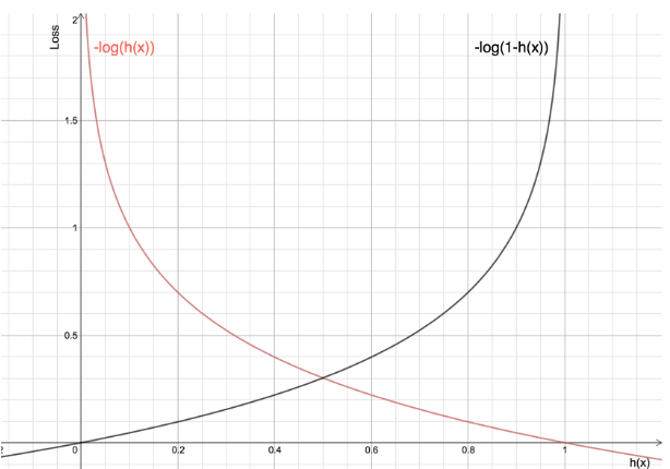
It gives rise to the exact same gradient descent updates as we saw for linear regression with MSE loss (see Section 5.9 for a derivation). We can now define the cost function for logistic regression by taking the average log-loss over all examples in the training set:
\[ J(\theta) = \frac{1}{M} \sum_{m=1}^M \textrm{Loss}(h_\theta(x^{(m)}), y^{(m)}) \]
Similar to linear regression, we can compute the update rule for gradient descent by setting the partial derivatives of \(J(\theta)\) to zero. We skip the derivation here, it is shows in Section 5.9. This yields the following update rules, which are basically the same update rules as for linear regression – except that here, we use the sigmoid function \(h_{\theta}\) This then gives rise to the gradient descent algorithm for logistic regression:
Here, \(h_\theta(x^{(m)}\) is the output \(\hat{y}\) (a real number between 0 and 1) of the logistic regressor on the \(m\)’th example \(x_m\), and \(y_m\) is the associated label.
For regression tasks, the Mean Squared Error (MSE) is one of the most common evaluation metric. For classification tasks, probably the most common evaluation metric is the proportion-correct accuracy, often abbreviated simply as Accuracy: it is the proportion of the examples that were correctly classified. With proportion-correct accuracy, higher numbers are better, whereas with MSE, lower numbers are better. Accuracy can be computed on either the training set or the test set. For instance, if the training set consists of 80 examples, and 65 of them were classified correctly by the machine, then the accuracy is \(65/80=0.8125\). Recall that the test accuracy indicates how well the trained machine will generalize, i.e., perform on unseen data on which it was not trained.
Interpreting the accuracy: When assessing whether a given accuracy is “good”, it is important to keep in mind how well you would do if you simply pick the dominant (most frequently occurring) class. This is sometimes called a “baseline” accuracy for guessing. Suppose a dataset consists of 90% positive examples and 10% negative examples. Then a machine that always outputs 1 (positive), irrespective of what its input \(x\) is, would trivially attain an accuracy of 90%. Hence, if your trained classifier achieves an accuracy similar to the baseline guessing accuracy, then it is not very useful.
We can use the LogisticRegression class of the sklearn.linear_model package to train a logistic regressor. In addition to the usual functions fit and predict that you’ve seen already, it also has a function predict_proba which outputs the probabilities of the input \(x\) belonging to each class. For binary classification, there are just two classes (e.g. 1 = heart pain, 0 = no heart pain), hence predict_proba will return a vector of two numbers: the first is \(P(y=0\ |\ x)\) and the second is \(P(y=1\ |\ x)\).
import numpy as np
import sklearn.linear_model

# Cholesterol levels of patients; need to ensure X is (M x 1) matrix.
X = np.atleast_2d([ 100, 233, 150, 280, 80, 320, 135, 93, 224, 178 ]).T
# Labels of whether they had heart pain in the next year
y = np.array([ 0, 1, 1, 1, 0, 1, 1, 0, 1, 0 ])

# Train model
logr = sklearn.linear_model.LogisticRegression()
logr.fit(X, y)

# We must pack the input x into a 2-d array of size (M x 1). Here, M=1.
yhat = logr.predict([ [ 190 ] ])  # gives 0/1 binary prediction
yhat_prob = logr.predict_proba([ [ 190 ] ])  # gives probabilistic prediction
print(yhat, yhat_prob)
[1] [[0.1643641 0.8356359]]As you can see, the binary prediction (from predict) for patient with cholesterol level 190 is that they will have heart pain (i.e., \(\hat{y}=1\)), and the probability (from predict_proba) that they will have pain is about 0.84. (Notice that the probabilities for all classes must always sum to 1.)
When using gradient descent to optimize a logistic regression model (or any other model for that matter), there are certain hyperparameters that influence how the training unfolds and thus how the trained model ultimately works. A hyperparameter is any variable that can influence the training process but that is not contained in the model itself; after the training has finished, the hyperparameters no longer have any relevance. The most common hyperparameters are the learning rate \(\alpha\) and the number of gradient descent iterations \(T\) – both of these can affect the final values of \(\theta_0,\theta_1,\ldots\) that are arrived at during training. Note that \(\theta_0,\theta_1,\ldots\) are not hyperparameters – they are the parameters of the model itself, and it’s the job of the training process to optimize them.
In the previous chapter, you saw how, if the learning rate \(\alpha\) is too low, then the cost function converges very slowly; on the other hand, if \(\alpha\) is too large, then the cost function might not converge at all (it could jump around, sometimes to infinity). So how do you choose a “good” \(\alpha\)? The most tempting strategy is simply to “pick the value that makes the test accuracy as high as possible”: for instance, you can try four different values for \(\alpha\), e.g. \(\alpha = 0.1, 0.01, 0.001, 0.0001\), train a model with each of these values of \(\alpha\), compute the accuracy of each model on the test set and pick the best one (with highest accuracy). However, that is not a proper approach, and if you follow it, you will almost certainly overestimate how good your trained model is.
The correct way to choose hyperparameters is to split your dataset into three disjoint (non-overlapping) parts – Training set, Validation set, and Test set – and to use them as follows:In most machine learning settings, you only have a finite set of data. Hence, you must decide how much data to apportion to each of subsets above. A typical “split” is around 80%, 10%, and 10% for training set, validation set, and test set.
Here’s an example of how the three subsets are used in practice: You typically first randomize the order of your data (to avoid dependencies between the data within each data subset) and then randomly partition the data into dataTrain, dataValid, and dataTest. Suppose we want to optimize the learning rate \(\alpha\) (a hyperparameter). Based on prior experimentation, reading papers, or asking colleagues, we might know that \(\alpha\) should be in the range \(0.0001\) and \(0.01\), but we don’t exactly what the best value is. A common strategy is to pick different values for \(\alpha\) within this range that are spaced apart by a power of 10, e.g., \(\alpha \in \{ 0.0001, 0.001, 0.01 \}\). We then proceed as follows:
bestAccuracy = -1
# Try each alpha
for alpha in [ 0.0001, 0.001, 0.01 ]:
    # Train on training data
    model = train(dataTrain, alpha)
    # Evaluate on validation data
    accuracy = evaluate(dataValid, model)
    # Keep track of best alpha
    if accuracy > bestAccuracy:
        bestAlpha = alpha
        bestAccuracy = accuracy
# Since we are done with hyperparameter search, it's
# legitimate to "add" the validation data to our training data
# (which tends to improve the accuracy on the test set).
bestModel = train(dataTrain + dataValid, bestAlpha)
accuracy = evaluate(dataTest, bestModel)
After training the bestModel, the hyperparameter \(\alpha\) is no longer needed. Note that, if there are multiple hyperparameters to optimize, then we would use nested loops to optimize their values jointly. For instance, if there is also a regularization strength hyperparameter \(\lambda\), then we could write:
bestAccuracy = -1
# Try each alpha
for alpha in [ 0.0001, 0.001, 0.01 ]:
    for lambda in [ .01, .1, 1 ]:
        # Train on training data
        model = train(dataTrain, alpha, lambda)
        # ...
Several built-in routines exist in Python and in the corresponding data science packages for hyperparameter optimization, based on approaches like grid search and Bayesian optimization.
Oftentimes in machine learning, there are more than 2 classes. For the face classification example, there might be multiple facial expressions, e.g., \(\{\textrm{smile}, \textrm{frown}, \textrm{neutral}, \textrm{sad}\}\). (Note: we are assuming here that each class is mutually exclusive, i.e., each face image \(x\) belongs to exactly one class – it cannot be both a smile and a frown.) For such problems, we can no longer apply logistic regression because that model is inherently built for binary classification. Instead, we must use a different approach. At a high level, there are two alternative strategies we can employ: (1) Decompose the multi-class problem (with \(K\) classes) into \(K\) different binary classification problems; or (2) Use an inherently multi-class classification technique such as softmax regressino or neural networks (which we will cover later in the course). We now discuss the first approach.
With one-vs-rest classification (sometimes also called one-vs-all classification), we train \(K\) binary classifiers. The goal of the \(k\)’th classifier (for \(k=1,\ldots,K\)) is to distinguish examples \(x\) that belong to class \(k\) from examples that belong to any class other than \(k\). For the set of four facial expressions listed above, we would thus train 4 binary classifiers: one that can tell whether a face is a smile versus anything other than a smile (i.e., frown, neutral, or sad); another one that can tell whether a face is a frown versus anything other than a frown; and so on. Each such binary classifier, when applied to a test image \(x\), gives the confidence \(\hat{y}\) of its prediction. To make a final determination as to the class of \(x\), we pick the class associated with the classifier whose prediction was most confident.
The figure below illustrates how this would be done for a setting with \(K=3\): We break up the 3-way classification problem into three 2-way (binary) classification problems: for each problem, we construct a separate training set with the corresponding binary labels and then train a model with it. Hence, in total we train \(K\) different binary classifiers. 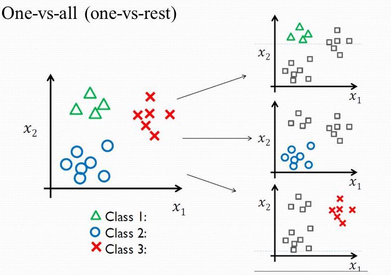
To obtain the label for a new example \(x\), we first apply each of the \(K\) binary classifiers to \(x\) to obtain \(\hat{y}_1, \hat{y}_2, \hat{y}_3\). These values express how likely the example \(x\) belongs to class \(k\). We then classify \(x\) according to which of the \(\hat{y}_k\) values is largest. For example, if \(\hat{y}_1=0.8, \hat{y}_2=0.7, \hat{y}_3=0.2\), then we classify \(x\) as class 1.
In the plots below you see some data points. You can imagine that the \(x\)-values might represent a person’s cholesterol level, and the \(y\)-values represent whether the person will have heart pain (\(y=1\), the positive class, means the patient does have heart pain, and \(y=0\), the negative class, means that they do not). Obviously, the higher the cholesterol, the higher the chance of heart pain. We could fit both a linear regression and a logistic regression model to this dataset; the fit models are shown below. The prediction curve \((x,h_\theta(x))\) is shown in blue for each model. For linear regression, it is a straight line, and for logistic regression it is the s-shaped sigmoid function \(g\). Moreover, the orange dotted vertical line shows the value \(x\) at which the model’s prediction is \(\hat{y}=0.5\) (equal chance of both classes). As you can see, both models arrive at approximately the same threshold (around \(x=150\)), and both models perfectly classify the entire dataset (i.e., to the right of the orange line, the data points all have \(y=1\), and to the left of the orange line, the data points all have \(y=0\).) 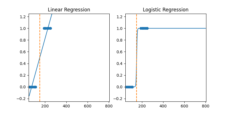
Now, however, suppose that there are some outliers/extreme values at the far right of the continuum. This corresponds to patients with a very high cholesterol level of around 800 (too much caviar!). Now you see how the two models (linear regression, logistic regression) give rise to different behaviors: the logistic model’s prediction line (blue) has hardly changed at all compared to the first scenario (without outliers). Why? Because the model was already classifying those new examples correctly, and there was thus no reason (in terms of the cost function) to change the parameters \(\theta\) very much. In contrast, the linear regression model is forced (via the MSE cost function) to adjust the prediction line considerably to accommodate the outliers. As a consequence, the value at which the prediction is \(\hat{y}=0.5\) has shifted to the left, which results in the model making some mistakes on a few of the examples (those just to the left of the prediction line whose label value \(y=1\)). 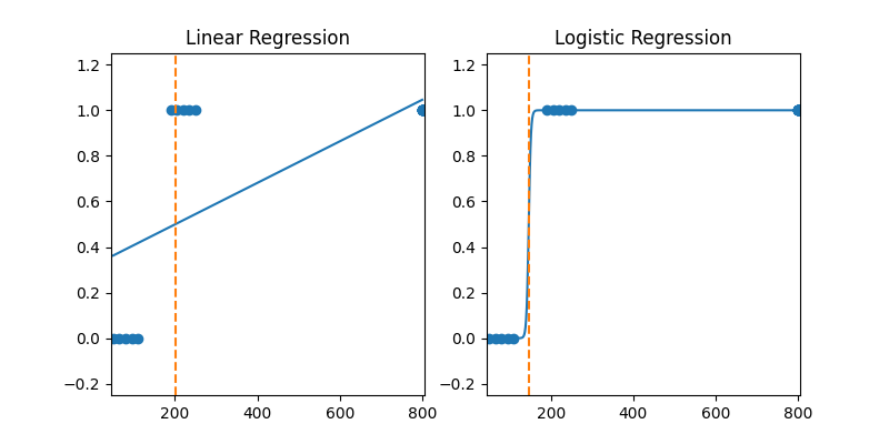
Below we derive the gradient descent updates for univariate logistic regression. We must find the partial derivative of the cost function \(J\) with respect to \(\theta_1\) and \(\theta_0\). Along the way, we need to use the fact that \(\frac{\partial}{\partial z} \log(z) = \frac{1}{z}\). Moreover, if \(z\) is a function of \(x\), then we have \(\frac{\partial}{\partial x} \log(z(x)) = \frac{1}{z(x)} \frac{\partial z}{\partial x}(x)\). Finally, we also use the identity that \(\frac{\partial}{\partial z} g(z) = g(z) (1 - g(z))\) (which can be shown by plugging in the definition for \(g\), calculating the derivative, and then simplifying).
\[\begin{eqnarray*} \frac{\partial}{\partial \theta_1} J(\theta_0, \theta_1) &=& - \frac{\partial}{\partial \theta_1} \left[ \frac{1}{M} \sum_{m=1}^M \left( y^{(m)} \log h_\theta(x^{(m)}) + (1-y^{(m)}) \log (1 - h_\theta(x^{(m)})) \right) \right] \\ &=& - \frac{1}{M} \sum_{m=1}^M \frac{\partial}{\partial \theta_1} \left( y^{(m)} \log g(\theta_0 + \theta_1 x^{(m)}) + (1-y^{(m)}) \log (1 - g(\theta_0 + \theta_1 x^{(m)})) \right) \\ &=& - \frac{1}{M} \sum_{m=1}^M \left( y^{(m)} \frac{\frac{\partial}{\partial \theta_1} g(\theta_0 + \theta_1 x^{(m)})}{g(\theta_0 + \theta_1 x^{(m)})} + (1-y^{(m)}) \frac{\frac{\partial}{\partial \theta_1} \left(1 - g(\theta_0 + \theta_1 x^{(m)}) \right)}{1 - g(\theta_0 + \theta_1 x^{(m)})} \right) \\ &=& - \frac{1}{M} \sum_{m=1}^M \left( y^{(m)} \frac{g(\theta_0 + \theta_1 x^{(m)})(1 - g(\theta_0 + \theta_1 x^{(m)}))x^{(m)} }{g(\theta_0 + \theta_1 x^{(m)})} - (1-y^{(m)}) \frac{g(\theta_0 + \theta_1 x^{(m)}) (1 - g(\theta_0 + \theta_1 x^{(m)}))x^{(m)} }{1 - g(\theta_0 + \theta_1 x^{(m)})} \right) \\ &=& - \frac{1}{M} \sum_{m=1}^M \left( y^{(m)} (1 - g(\theta_0 + \theta_1 x^{(m)}))x^{(m)} - (1-y^{(m)}) g(\theta_0 + \theta_1 x^{(m)})x^{(m)} \right) \\ &=& - \frac{1}{M} \sum_{m=1}^M \left( y^{(m)} - y^{(m)} g(\theta_0 + \theta_1 x^{(m)}) - g(\theta_0 + \theta_1 x^{(m)}) + y^{(m)} g(\theta_0 + \theta_1 x^{(m)}) \right) x^{(m)} \\ &=& - \frac{1}{M} \sum_{m=1}^M \left( y^{(m)} - g(\theta_0 + \theta_1 x^{(m)}) \right) x^{(m)} \\ &=& \frac{1}{M} \sum_{m=1}^M ( h_\theta(x^{(m)}) - y^{(m)}) x^{(m)} \\ \end{eqnarray*}\]
The derivation of \(\frac{\partial}{\partial \theta_0} J(\theta_0, \theta_1)\) turns out to be very similar, except that there is no \(x^{(m)}\) in the result:
\[\begin{eqnarray*} \frac{\partial}{\partial \theta_0} J(\theta_0, \theta_1) &=& \frac{1}{M} \sum_{m=1}^M (h_\theta(x^{(m)}) - y^{(m)}) \end{eqnarray*}\]
If you compare the gradient descent updates for logistic regression (with the log loss) to those for linear regression (with RSS loss), you can see they are exactly the same.