6 Support Vector Machines

The following discussion makes use of the term dimension and space. Note that these dimensions (denoted \(x_1\), \(x_2\), \(x_3\), …) correspond to features in the dataset at hand, that is columns in the matrix \(\mathbf{X}\) introduced in Section 1.3. So the scatterplots of data samples \(\{(x_1^{(1)}, x_2^{(1)}), (x_1^{(2)}, x_2^{(2)}), \dots, (x_1^{(M)}, x_2^{(M)})\}\) imply, that the respective datasets have two features, i.e. \(N=2\).

The binary classification setting involves \(M\) training samples in \(N\)-dimensional space,

\[\mathbf{x}^{(1)}=\begin{pmatrix}x_1^{(1)} \\ \vdots \\ x_N^{(1)}\end{pmatrix}, \dots, \begin{pmatrix}x_1^{(M)} \\ \vdots \\ x_N^{(M)}\end{pmatrix},\]

with associated class labels \(y^{(1)}, y^{(2)}, \dots , y^{(M)} \in \{−1, +1\}\), where \(−1\) represents one class and \(+1\) the other class instead of \(\{0,1\}\), which makes some derivations more convenient.
A test sample is denoted as \(\mathbf{x}^{\ast} = \begin{pmatrix}x_1^{(\ast)} & \dots & x_N^{(\ast)}\end{pmatrix}^T\). The goal is to develop a classifier based on the training data that will correctly classify the test sample.

6.1 Hyperplanes and the Maximal Margin Classifier

In \(N\)-dimensional space, a hyperplane is a flat affine¹ subspace of dimensions \(N−1\). For instance, in two dimensions, a hyperplane is a one-dimensional subspace - a line, as can be seen in Figure 6.1. In three dimensions, a hyperplane is a flat two-dimensional subspace — a plane. In \(N>3\) dimensions, it can be hard to visualize a hyperplane, but the notion of a (\(N−1\))-dimensional flat subspace still applies.
In two dimensions, a hyperplane is defined by the equation

\[b + w_1 x_1 + w_2 x_2 = 0 \tag{6.1}\]

for parameters \(b\), \(w_1\),and \(w_2\). Any \(\mathbf{x}=\begin{pmatrix}x_1 & x_2\end{pmatrix}^T\) for which Equation 6.1 holds is a point on the hyperplane (in this case a line, see Figure 6.1).
The formulation can be easily extended to the \(N\)-dimensional setting:

\[b + w_1 x_1 + w_2 x_2 + \dots + w_N x_N = 0 \tag{6.2}\]

defines a \(N\)-dimensional hyperplane, again in the sense that if a point \(\mathbf{x}=\begin{pmatrix}x_1 & x_2 & \dots & x_N\end{pmatrix}^T\) in \(N\)-dimensional space (i.e. a vector of length \(N\)) satisfies Equation 6.3, then \(\mathbf{x}\) lies on the hyperplane. Also the \(w\)’s can be expressed as a \(N\)-dimensional parameter vector and the scalar (dot) product \(\langle\mathbf{w},\mathbf{x}\rangle=\mathbf{w}^T\mathbf{x} = \sum_{n=1}^N w_n x_n\) allows to express Equation 6.3 in compact form:

\[b + \mathbf{w}^T\mathbf{x} = 0 \tag{6.3}\]

This “\(w\), \(b\)” notation allows us to explicitly treat the intercept term \(b\) separately from the other parameters \(\{w_n\}\). Also, the convention used in linear and logistic regression of letting \(x_0 = 1\) be an extra coordinate in the input feature vector is not used here. Thus, \(b\) takes the role of what was previously \(\theta_0\), and \(\mathbf{w}\) takes the role of \(\begin{pmatrix}\theta_1 \dots \theta_n\end{pmatrix}^T\).

Now, suppose that \(\mathbf{x}\) does not satisfy Equation 6.3; rather,

\[b + \mathbf{w}^T\mathbf{x} > 0.\]

Then this tells us that \(\mathbf{x}\) lies on one side of the hyperplane. On the other hand, if

\[b + \mathbf{w}^T\mathbf{x} < 0,\]

then \(\mathbf{x}\) lies on the other side of the hyperplane. So we can think of the hyperplane as dividing the \(N\)-dimensional space into two parts. One can easily determine on which side of the hyperplane a point lies by simply calculating the sign of the left hand side of Equation 6.3.

Figure 6.1: An example for a hyperplane in 2-dimensional feature space. That is, when our dataset comprises two features \(x_1\) and \(x_2\). The hyperplane \(1+2x_1+3x_2=0\) is shown as a black solid line. The blue region is the set of points for which \(1+2x_1+3x_2>0\) and the red region is the set of points for which \(1+2x_1+3x_2<0\).

Suppose that it is possible to construct a hyperplane that separates the training samples perfectly according to their class labels. Examples of three such separating hyperplanes are shown in Figure 6.2 (a).

(a) Three separating hyperplanes, out of many possible, are shown in black.

The goal of the learning algorithm is to find the optimal values \(\hat{\mathbf{w}}\) and \(\hat{b}\) for parameters \(\mathbf{w}\) and \(b\). Once the learning algorithm has identified these optimal values, some new input feature vector \(\mathbf{x}^{(\ast)}\) can be classified by:

\[f(\mathbf{x}^{\ast})= \hat{b} + \hat{\mathbf{w}}^T\mathbf{x}^{(\ast)}\]

If \(f(\mathbf{x}^{\ast})\) is positive, the test sample is assigned to class \(+1\), and if \(f(\mathbf{x}^{\ast})\) is negative, then it is assigned to class \(−1\) (compare Figure 6.2 (b)).
The magnitude of \(f(\mathbf{x}^{\ast})\) encodes the confidence with which the class label was assigned. If \(f(\mathbf{x}^{\ast})\) is far from zero, then this means that \(\mathbf{x}^{\ast}\) lies far from the hyperplane, and so we can be confident about our class assignment for \(\mathbf{x}^{\ast}\). On the other hand, if \(f(\mathbf{x}^{\ast})\) is close to zero, then \(\mathbf{x}^{\ast}\) is located near the hyperplane, and so we are less certain about the class assignment for \(\mathbf{x}^{\ast}\).

\(\hat{\mathbf{w}}\) and \(\hat{b}\) are found by solving a constrained optimisation problem: The hyperplane should separate positive examples from negative ones with the largest margin. A large margin contributes to a better generalisation, that is how well the model will classify new examples once it is trained. Figure 6.3 shows the maximal margin hyperplane (solid line) on the data set of Figure 6.2. The margin is the prependicular distance from the hyperplane to the closest examples of the two classes - the so called support vectors, indicated by black circles. These are vectors in \(N\)-dimensional space (in Figure 6.3, \(N=2\)) and they “support” the maximal margin hyperplane in the sense that if these points were moved slightly then the maximal margin hyperplane would move as well.

In a sense, the maximal margin hyperplane represents the mid-line of the widest street that can be drawn between the two classes. The two margin boundaries (grey dashed lines) are therefore also called gutters. They correspond to two hyperplanes satisfying the equations

\[\hat{b} + \hat{\mathbf{w}}^T\mathbf{x}=1\] \[\hat{b} + \hat{\mathbf{w}}^T\mathbf{x}=-1\]

The distance between these two hyperplanes is given by \(\frac{2}{||\mathbf{w}||}\), so the smaller the norm of the parameter vector \(||\mathbf{w}||\), the larger the distance between these two hyperplanes. This is the minimisation objective.

At the same time, the following constraints ensure that each training sample is on the correct side of the hyperplane:

\[b + \mathbf{w}^T\mathbf{x}^{(m)} > 0 \ \ \ \text{if} \ y^{(m)}=1, \tag{6.4}\]

and

\[b + \mathbf{w}^T\mathbf{x}^{(m)} < 0 \ \ \ \text{if} \ y^{(m)}=-1 \tag{6.5}\]

This can be expressed equivalently in a more compact form:

\[y^{(m)} \left(b + \mathbf{w}^T\mathbf{x}^{(m)}\right) > 0 \tag{6.6}\]

So the final constraint minimisation problem is:

\[\underset{b, \mathbf{w}}{\text{min}}\frac{1}{2}||\mathbf{w}||^2 \tag{6.7}\]

\[\text{subject to} \ y^{(m)}\left(b + \mathbf{w}^T\mathbf{x}^{(m)} \right) \geq 1 \ \forall \ m=1,\dots,M \tag{6.8}\]

The factor \(\frac{1}{2}\) in the minimisation is introduced for mathematical convenience and does not influence the solution.

Interestingly, the maximal margin hyperplane defined by \(b,\mathbf{w}\) depends directly on the support vectors, but not on the other samples: A movement to any of the other samples would not affect the separating hyperplane, provided that the sample’s movement does not cause it to cross the boundary set by the margin.

Naturally, a classifier that is based on a separating hyperplane leads to a linear decision boundary.

Figure 6.3: There are two classes of samples, shown in blue and in red. The maximal margin hyperplane is shown as a solid line. The margin is the distance from the solid line to either of the dashed lines. The two blue points and the red point that lie on the dashed lines are the support vectors, and the distance from those points to the hyperplane is indicated by grey solid lines. The red and blue grid indicates the decision rule made by a classifier based on this separating hyperplane.

Because the maximal margin classifier does not allow any violation of the separating hyperplane (each sample has to be on the correct side), it is also called hard margin classifier - as opposed to the soft margin classifier, which is discussed in the following section.

6.2 Soft Margin Classifier

Figure 6.4: There are two classes of samples, shown in blue and in red. In this case, the two classes are not separable by a hyperplane, and so the maximal margin classifier cannot be used.

In many cases no separating hyperplane exists, that is, the optimization problem has no solution. An example is shown in Figure 6.4. In this case, the two classes cannot be separated exactly.
In fact, even if a separating hyperplane does exist, a hard margin classifier might not always be desirable. A classifier based on a separating hyperplane will necessarily perfectly classify all of the training samples; this can lead to sensitivity to individual samples or outliers. An example is shown in Figure 6.5. The addition of a single sample in Figure 6.5 (b) leads to a dramatic change in the maximal margin hyperplane. The resulting maximal margin hyperplane is not satisfactory - for one thing, it has only a tiny margin. This is problematic because the distance of an sample from the hyperplane can be seen as a measure of the confidence that the sample was correctly classified. Moreover, the fact that the maximal margin hyperplane is extremely sensitive to a change in a single sample suggests that it may have overfit the training data.
In this case, a classifier based on a hyperplane that does not perfectly separate the two classes might be a better choice in the interest of

greater robustness to individual samples, and
better generalisability.

That is, it could be worthwhile to misclassify a few training samples in order to better classify the remaining samples. The soft margin classifier (also called support vector classifier) as an extension to the maximal margin classifier does exactly this. The margin is called soft because it is allowed to be violated by some of the training samples.

(a) A dataset consisting of two classes of samples, shown in blue and in red, and two variables (features), along with the maximal margin hyperplane as a solid line

Figure 6.6 (a) shows an example for a soft margin classifier. Most of the samples are on the correct side of the margin. However, a small subset of the samples are on the wrong side of the margin. An sample can be not only on the wrong side of the margin, but also on the wrong side of the hyperplane. In fact, when there is no separating hyperplane, such a situation is inevitable. Samples on the wrong side of the hyperplane correspond to training samples that are misclassified by the support vector classifier. Figure 6.6 (b) illustrates such a scenario.

(a) Red samples 3, 4, 5 and 6 are on the correct side of the margin, sample 2 is on the margin, and sample 1 is on the wrong side of the margin. Blue samples 7 and 10 are on the correct side of the margin, sample 9 is on the margin and sample 8 is on the wrong side of the margin. No samples are on the wrong side of the hyperplane.

For the soft margin classifier slack variables \(\mathbf{\epsilon}=\begin{pmatrix}\epsilon_1 & \epsilon_2 & \dots & \epsilon_M\end{pmatrix}^T, \epsilon_m\geq0\) are introduced. They allow a few individual samples to be on the wrong side of the margin. The larger their value, the further the respective sample reaches onto the wrong side of the margin (\(\epsilon_m > 0\)). They can be even on the wrong side of the hyperplane (\(\epsilon_m > 1\)).
The hard constraint that \(y^{(m)}f(\mathbf{x}^{(m)}) \geq 0\) is replaced by the soft margin constraint that \(y^{(m)}f(\mathbf{x}^{(m)}) \geq 1-\epsilon_m\). The new objective becomes

\[\underset{b, \mathbf{w}, \mathbf{\epsilon}}{\text{min}}\frac{1}{2}||\mathbf{w}||^2 + C \sum_{m=1}^M\epsilon_m \tag{6.9}\] \[\text{subject to }\epsilon_m \geq0, \ y^{(m)}\left( b + \mathbf{w}^T\mathbf{x}^{(m)} \right) \geq 1-\epsilon_m \tag{6.10}\]

where \(C\) is nonegative and acts as a regularisation parameter. It controls how many points are allowed to violate the margin constraint. Here, the samples that either lie on the margin or that violate the margin are the support vectors. Equivalent to the hard margin classifier, only the support vectors affect the hyperplane, and hence the resulting soft margin classifier. A sample that lies strictly on the correct side of the margin does not affect the soft margin classifier! Changing the position of that sample would not change the classifier at all, provided that its position remains on the correct side of the margin.
The value of \(C\) affects the bias-variance trade-off of the model: When \(C\) is small, the margin is wide, many samples may violate the margin, and so there are many support vectors which determine the hyperplane - see Figure 6.7 (a), where essentially all samples are support vectors. This amounts to fitting the data less hard and obtaining a classifier with low variance but potentially high bias.
In contrast, if \(C\) is large, narrow margins are prefered that are rarely violated. So there will be fewer support vectors. Figure 6.7 (d) illustrates this setting, with only 10 support vectors. This amounts to a classifier that is highly fit to the data, which may have low bias but high variance. \(C=\infty\) reduces to the unregularised, hard-margin classifier - of course, a maximal margin hyperplane exists only if the two classes are separable.

In practice, \(C\) is treated as a tunable hyperparameter that is generally chosen via cross-validation.

6.3 Support Vector Machines and the Kernel-Trick

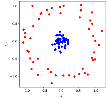
Many classification problems are not linearly separable, such as the data in Figure 6.8 (a). It is clear that a support vector classifier or any linear classifier will perform poorly here.

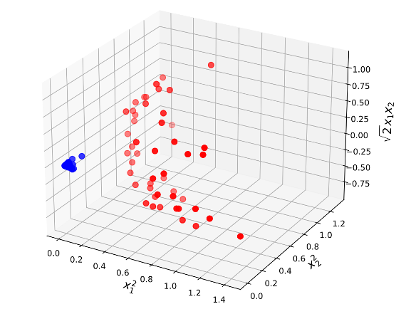
However, in many cases the original space can be transformed into a space of higher dimensionalty, where the examples become linearly separable. This effect is illustrated in Figure 6.8 using a transformation \(\phi: \mathbf{x} \rightarrow \phi\left(\mathbf{x}\right)\)

\[\phi \begin{pmatrix}x_1 \\ x_2\end{pmatrix}=\begin{pmatrix}x_1^2 \\ \sqrt{2}x_1 x_2 \\ x_2^2\end{pmatrix}\]

However, many different transformations are possible and it is hard to know a priori which one will work for a given dataset. Considering through many transformations explicitly is computationally very inefficient.

kernels (kernel functions) are the solution to this dilemma. They allow to efficiently work in higher-dimensional spaces without going through the transformations explicitly.

We have not discussed, how the minimisation Equation 6.9 and Equation 6.10 is actually solved. Typically, the original (primal) problem, is recast in an equivalent dual problem using the method of Lagrange multipliers:

\[ \max\mathcal{L}(\alpha) = -\frac{1}{2} \sum_{i=1}^{M} \sum_{j=1}^{M} \alpha_i \alpha_j y^{(i)} y^{(j)} \mathbf{x}^{(i)} \mathbf{x}^{(j)} + \sum_{m=1}^{M} \alpha_m \tag{6.11}\]

subject to

\[ \sum_{m=1}^{M} \alpha_m y^{(m)} = 0 \quad \text{and} \quad 0 \leq \alpha_m \leq C \quad \text{for} \quad m = 1, \ldots, M \]

where \(\alpha_i\) are the Lagrange multipliers. This form represent a quadratic optimisation problem which can be solved efficiently by dedicated algorithms.

The only place, where the feature vectors are used in Equation 6.11 is the term \(\mathbf{x}^{(i)} \mathbf{x}^{(j)}\). A transformation into a higher dimensional space would imply transforming all \(\mathbf{x}^{(i)}\) into \(\phi\left(\mathbf{x}^{(i)}\right)\) and \(\mathbf{x}^{(j)}\) into \(\phi\left(\mathbf{x}^{(j)}\right)\), respectively. Doing so explicitly is computationally demanding.
However, actually the formula only uses the scalar product \(\mathbf{x}^{(i)} \mathbf{x}^{(j)}\), which is a real number. By using the kernel trick, the explicit transformation of the individual feature vectors and calculation of the scalar product can be circumvented. It is replaced by a simpler operation on the original feature vectors that gives the same result. For example:

Instead of transforming

\(\begin{pmatrix}x_1^{(i)} \\ x_2^{(i)}\end{pmatrix}\) into \(\begin{pmatrix}(x_1^{(i)})^2 \\ \sqrt{2}x_1^{(i)} x_2^{(i)} \\ (x_2^{(i)})^2\end{pmatrix}\)

and \(\begin{pmatrix}x_1^{(j)} \\ x_2^{(j)}\end{pmatrix}\) into \(\begin{pmatrix}(x_1^{(j)})^2 \\ \sqrt{2}x_1^{(j)} x_2^{(j)} \\ (x_2^{(j)})^2\end{pmatrix}\)

and then computing the scalar product

\[\begin{pmatrix}(x_1^{(i)})^2 \\ \sqrt{2}x_1^{(i)} x_2^{(i)} \\ (x_2^{(i)})^2\end{pmatrix} \cdot \begin{pmatrix}(x_1^{(j)})^2 \\ \sqrt{2}x_1^{(j)} x_2^{(j)} \\ (x_2^{(j)})^2\end{pmatrix} = (x_1^{(i)})^2 (x_1^{(j)})^2 +2 x_1^{(i)}x_1^{(j)}x_2^{(i)}x_2^{(j)}+(x_2^{(i)})^2 (x_2^{(j)})^2,\]

the scalar product of the original feature vectors:

\[ \begin{pmatrix}x_1^{(i)} \\ x_2^{(i)}\end{pmatrix} \cdot \begin{pmatrix}x_1^{(j)} \\ x_2^{(j)}\end{pmatrix} = \left(x_1^{(i)} x_1^{(j)} + x_2^{(i)}x_2^{(j)}\right)\]

can be computed directly and then squared to get the same result. This results in much fewer and more efficient computations.

This is an example of the kernel trick, which generally consists of replacing a scalar product by a kernel function

\[\mathcal{K}(\mathbf{x}^{(m)},\mathbf{x}^{(m')}), \tag{6.12}\]

which quantifies the similarity of two samples. The linear kernel

\[\mathcal{K}(\mathbf{x}^{(m)},\mathbf{x}^{(m')}) = \sum_{n=1}^N x^{(m)}_n x^{(m')}_n \tag{6.13}\]

for instance, would just result in the support vector classifier. In the example above a quadradic kernel

\[\mathcal{K}(\mathbf{x}^{(m)},\mathbf{x}^{(m')})=\left(\sum_{n=1}^N x^{(m)}_n x^{(m')}_n\right)^2 \tag{6.14}\]

was used. The more general form is the polynomial kernel:

\[\mathcal{K}(\mathbf{x}^{(m)},\mathbf{x}^{(m')})=\left(1+\sum_{n=1}^N x^{(m)}_n x^{(m')}_n\right)^d \tag{6.15}\]

where the degree \(d\) is a positive integer. Using such a kernel with \(d>1\), instead of the standard linear kernel Equation 6.13, in the support vector classifier algorithm leads to a much more flexible decision boundary. When the support vector classifier is combined with a non-linear kernel such as Equation 6.15, the resulting classifier is known as a support vector machine. Figure 6.9 (c) shows an example of an SVM with a polynomial kernel applied to a non-linearly separable dataset. The fit is a substantial improvement over the linear support vector classifier Figure 6.9 (b).

Another popular choice for a non-linear kernel function is the rbf kernel (rbf: short for Radial Basis Function, also just called radial or Gaussian kernel):

\[\mathcal{K}\left(\mathbf{x}^{(m)},\mathbf{x}^{(m')}\right)=\exp\left(-\gamma ||\mathbf{x}^{(m)} -\mathbf{x}^{(m')}||^2 \right), \tag{6.16}\]

Figure 6.9 (d) shows an SVM with a rbf-kernel applied to the non-linearly separable data from Figure 6.9 (a).

\(\gamma\) in Equation 6.16 is a positive constant inversely proportional to the variance of the Gaussian \(\gamma=\frac{1}{\sigma^2}\). That is, with larger values for \(\gamma\) (smaller variance \(\sigma^2\)) the Kernel has a smaller spread and influences the classification only in the immediate surrounding of each sample. This makes the decision boundary typically rougher - leading to low bias, but high variance (a small change in the data has a large effect).
Smaller values for \(\gamma\), on the other hand, lead to a larger spread of the Kernel and the classification in a given point in space is influenced by more distant samples, which partially level each other out. This makes the decision boundary smoother - leading to lower variance, but high bias.

\(\gamma\) and \(d\) are hyperparameters that are typically tuned along with \(C\) via cross-validation.

(a) A classification dataset consisting of blue and red samples with a non-linear boundary between the two classes.

6.4 SVMs With More Than Two Classes

The SVM is formulated per se as a binary classification problem. It turns out that the concept of separating hyperplanes can not readily be extended to more than two classes \(K>2\). However, the one-versus-all and one-vs-one approaches can be employed.

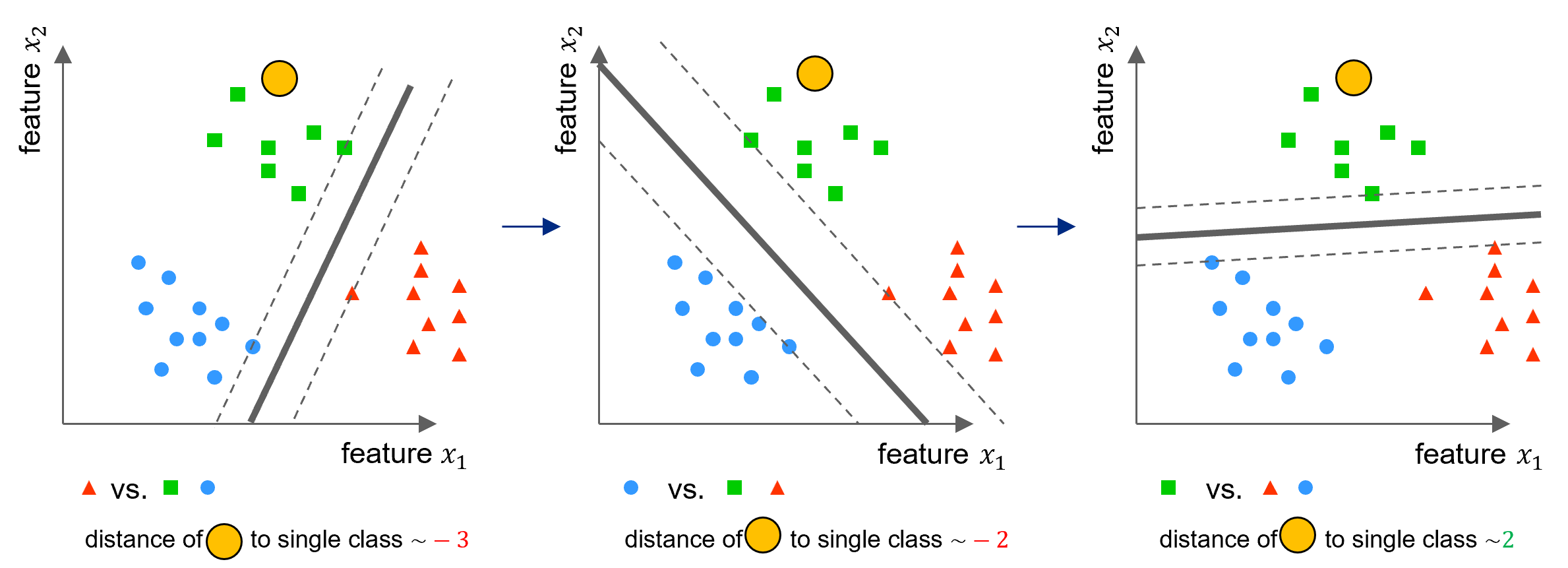
The one-vs-all (or one-vs-rest) approach is described in Section 5.7.1. \(K\) SVMs are fitted, each one classifying one of the \(K\) classes to the remaining \(K-1\) classes. Let \(b_k,w_{1k},\dots,w_{Nk}\) denote the parameters that result from fitting an SVM comparing the \(k\)th class (coded as \(+1\)) to the others (coded as \(−1\)). Let \(\mathbf{x}^{(\ast)}\) denote a test sample (yellow in Figure 6.10). We assign the sample to the class for which \(f(\mathbf{x}^{\ast})= b_k + \mathbf{w}_k^T\mathbf{x}^{(\ast)}\) is largest, as this amounts to a high level of confidence that the test sample belongs to the \(k\)th class rather than to any of the other classes.

Figure 6.10: Illustration of the one-vs-all scheme applied to 3 classes in colors red, blue and green. With the unknown test sample in yellow

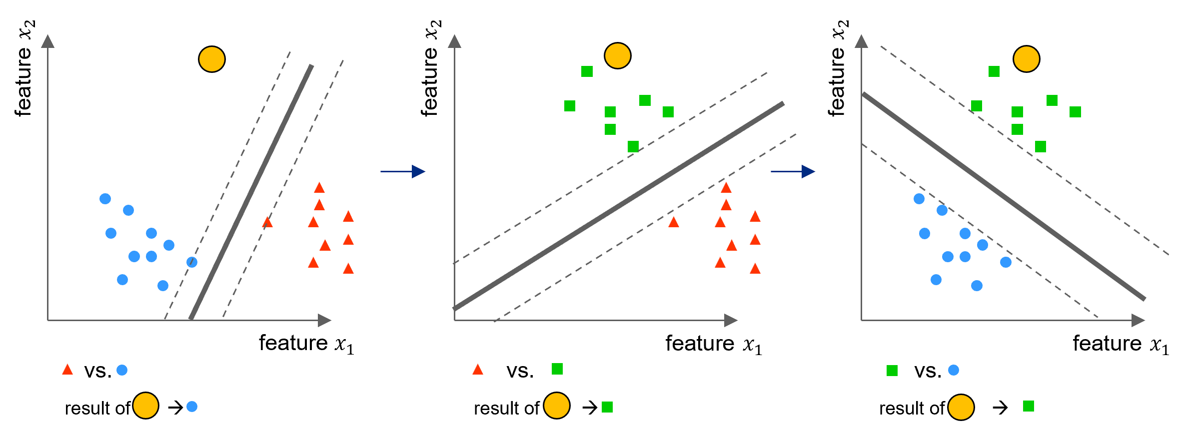
In the one-versus-one approach a separate SVM is constructed for each of the \(\binom{K}{2}\) distinct pairs of classes Figure 6.11. A test sample is classified using each of the classifiers and the number of times that the test sample is assigned to each of the \(K\) classes is counted. The test sample is the assigned to the class to which it was most frequently assigned in those pairwise classifications (majority vote).

Figure 6.11: Illustration of the one-vs-one scheme applied to 3 classes in colors red, blue and green. The unknown test instance (yellow) is assigned by majority vote

6.5 SVMs for Regression

To use SVMs for regression instead of classification, the trick is to tweak the objective: Instead of trying to fit the largest possible street between two classes while limiting margin violations, SVM regression tries to fit as many instances as possible on the street while limiting margin violations (i.e., instances off the street). The width of the street is controlled by a hyperparameter, \(\epsilon\). Figure 6.12 shows two linear SVM regression models trained on some linear data, Figure 6.12 (a) with a small margin and Figure 6.12 (b) with a larger margin.

Reducing \(\epsilon\) increases the number of support vectors, which regularizes the model. Moreover, if more training instances within the margin are added, it will not affect the model’s predictions; thus, the model is said to be \(\epsilon\)-insensitive.

To tackle nonlinear regression tasks, kernelized SVM models can be employed. Figure 6.13 shows SVM regression on a random quadratic training set, using a second-degree polynomial kernel. There is some regularization in Figure 6.13 (a) (i.e., a small \(C\) value), and much less in Figure 6.13 (b) (i.e., a large \(C\) value).

The subspace does not need to pass through the origin.↩︎