1 Introduction
We start with some fundamental terminology and high level concepts to get you started…
1.1 Machine Learning
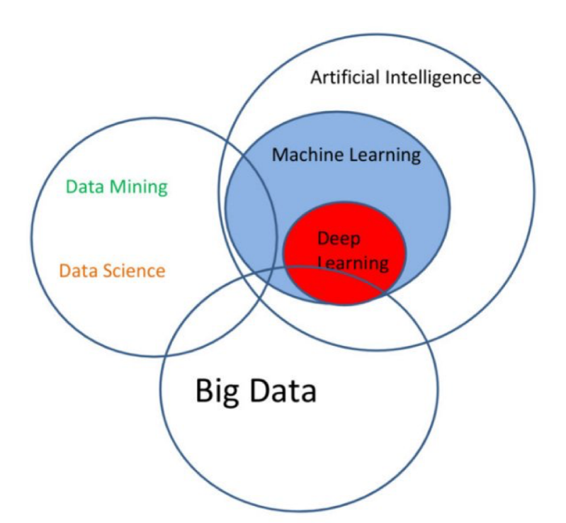
Machine Learning (ML) is a branch of artificial intelligence (AI) devoted to developing and understanding methods that “learn”, i.e. that…
… leverage data to make predictions or decisions (act like humans) without being explicitly programmed to do so. (Arthur Samuel, Wikipedia)
Model: A model is a logical, mathematical or probabilistic relationship between several variables.
Learning (also called Training): Machine Learning employs adaptive models, which are configured and parameterised automatically based on the training data.
The computational methods in Machine learning are used to discover patterns in the data and/or to derive a corresponding generating process to
- gain insights and
- predict events
in order
- provide a quantitative basis for decisions (actionable insights), e.g. determine target segments for marketing campaigns, or
- to influence the underlying process of the data, e.g. adapt the user features of an app.
Deep Learning is a a subset of machine learning that employs Deep Neural Networks, which are models inspired by the neurons in the human brain.
1.2 Machine Learning Paradigms
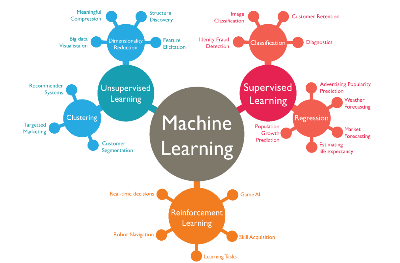
The three main machine learning paradigms are Supervised Learning, Unsupervised Learning, and Reinforcement Learning. We will now briefly describe these paradigms.
1.3 Supervised Learning
In Supervised Learning, we use a dataset with annotated training samples to “teach” a machine to perform a certain task.
Example. Assume we want to recognize the sentiment of a sentence, i.e. whether the sentence contains a positive or negative emotion, or whether it is neutral. For instance, the sentence “This is a nice car” is positive, whereas “He is 35 years old” is neutral. For this, we could create a (large) set of Annotated (or Labeled) Training Samples, i.e. a set of sentences where we annotate for each sentence its sentiment. Then, we can use a machine learning algorithm to learn from this Training Dataset. A classical algorithm would first extract some Features from each text, e.g. the text length, the number of positive and negative words, the number of exclamation marks, the number of negation words etc. These features are then used to build a mathematical model which determines which combination of features typically indicate a certain sentiment of the text (e.g. a short text with one positive word and one negation word, and thus has probably negative sentiment, as in “This is not nice”).
We now describe this idea in a more abstract way: Let’s consider a setting where we extract \(N\) features for each training sample, and where our training dataset \(X\) contains \(M\) training samples. In addition, we have for each training sample its label (the sentiment of each training sentence in the example above), which is stored in a vector \(y\) of length \(M\). Thus, we have:
Dimension of \(X\): \(M \times N\)
Dimensions of \(y\): \(M\)
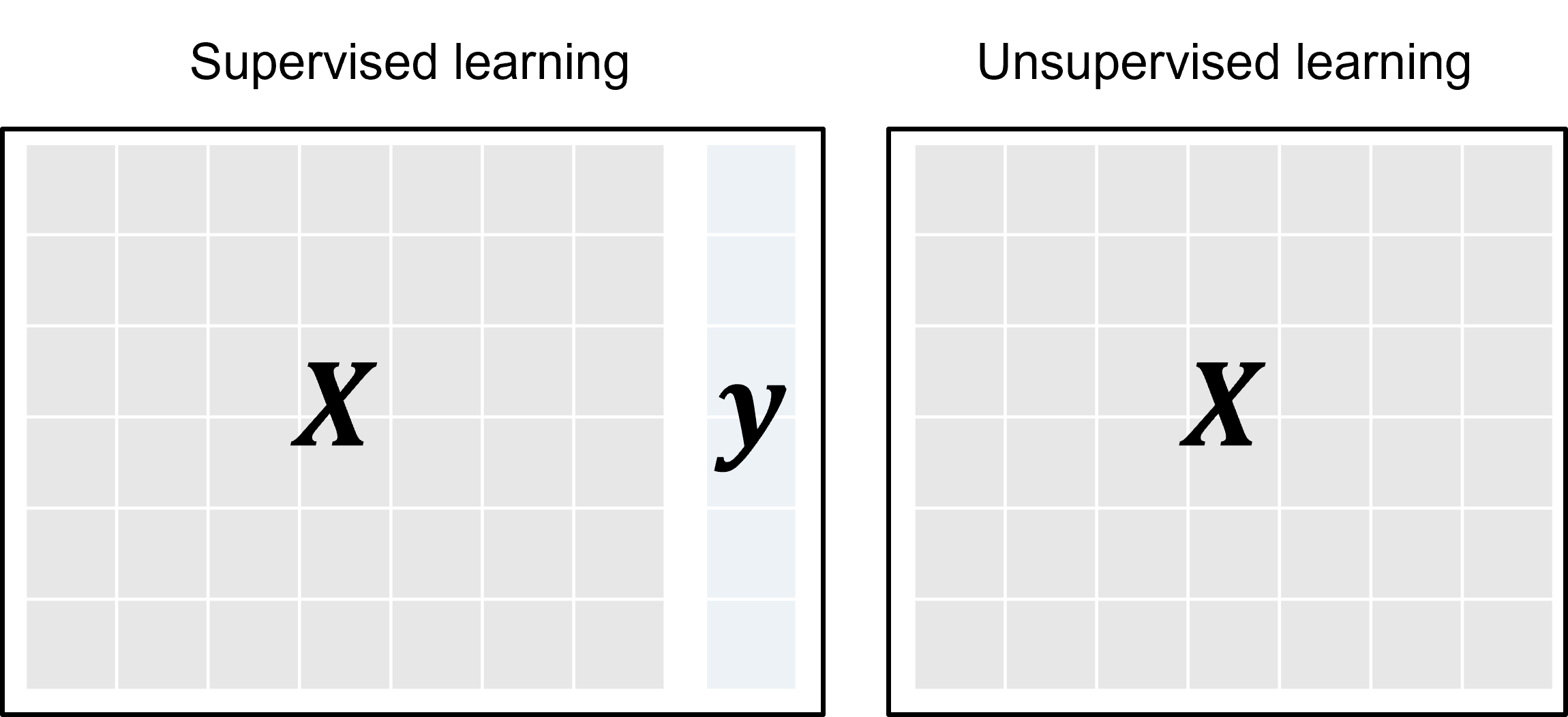
Thus, the training data consists of \(M\) input samples \(𝑋_{𝑚,:}\) (rows in the matrix \(X\)) and their associated output values \(𝑦^{(m)}\) (note that we denote single samples with superscript \(^{(m)}\)). Note that in Unsupervised Learning, we would only have the sample set \(X\), but no labels \(y\) for the samples.
In supervised learning we try to find a function \(𝑓\) which systematically produces the output values \(𝑦^{(𝑚)}\) associated with the input values \(𝑿_{𝑚,:}\) per sample \(m\): \(𝑓(𝑿_{𝑚,:})\rightarrow 𝑦^{(m)}\). An equivalent notation for a single data instance (one row on figure 1.3., left) is \(𝑓(x^{(m)}_:)\rightarrow 𝑦^{(m)}\), which indicates the \(m-\)th data sample, including all its dimensions, denoted here with “\(:\)”. Supervised learning aims to find a mapping from input data to their corresponding outputs.
The columns of \(X\) represent the Features, which are also called Independent Variables, Predictors, Attributes or Covariates. Inputs can vary widely depending on the application: can be tabular data (properties of a car like mileage, age, brand), text (product reviews), images (object detection) which are converted to numerical format. The associated output values \(𝑦^{(m)}\) are individual observations of the target variable, also called response variable. In classification settings these values are also called Labels.
There exist numerous algorithms for supervised learning, e.g. Support Vector Machines, Logistic Regression, Decision Trees, or Deep Neural Networks.
1.4 Unsupervised Learning
In Unsupervised Learning the training data does not contain any expected output values. The goal is to model the underlying distribution of the data \(X\) (describe the structure of the data), in order to explain it and to apply the model to new data. This brings additional challenges compared to supervised learning:
- The problem statement is much fuzzier
- The evaluation is more difficult without test data including expected output values
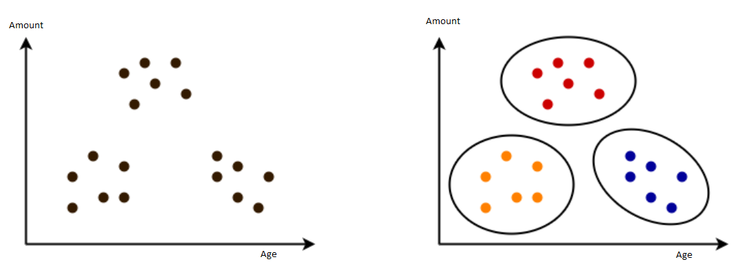
Example: Clustering is the task of grouping a set of objects in such a way that objects in the same group (called a Cluster) are more similar (in some sense) to each other than to those in other groups (clusters). Assume, for instance, that we collect for customers in a shop their age and the amount they spend in the shop. Then we might get the image below, left side. Based on this information, a clustering algorithm such as K-Means might group these customers into three groups, as shown on the right side. We can now see, for instance, that there is a group of young people and a group of elder people who spend little, while a group of mid-aged people spends a lot. (Obviously, this is a trivial example which could have been done easily by hand; however, assume that we do not only collect 2 features (age and amount), but hundreds of features of thousands of customers, then doing the clustering by hand becomes infeasible.)
1.5 Reinforcement Learning
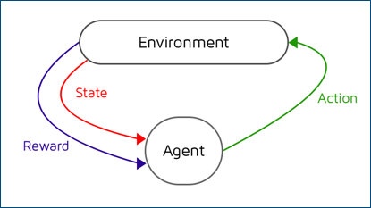
In Reinforcement Learning, the learning system, called an Agent in this context, can observe the Environment, select and perform Actions, and get Rewards in return (or penalties in the form of negative rewards), as shown in Figure 1.5. It must then learn by itself what is the best strategy, called a Policy, to get the most reward over time. A policy defines what action the agent should choose when it is in a given situation.
1.6 Details of Supervised Learning
We now discuss some typical methods and technologies of supervised learning.
1.6.1 Classification vs. Regression
Supervised learning problems are distinguished regarding the type of the target variable \(y\).
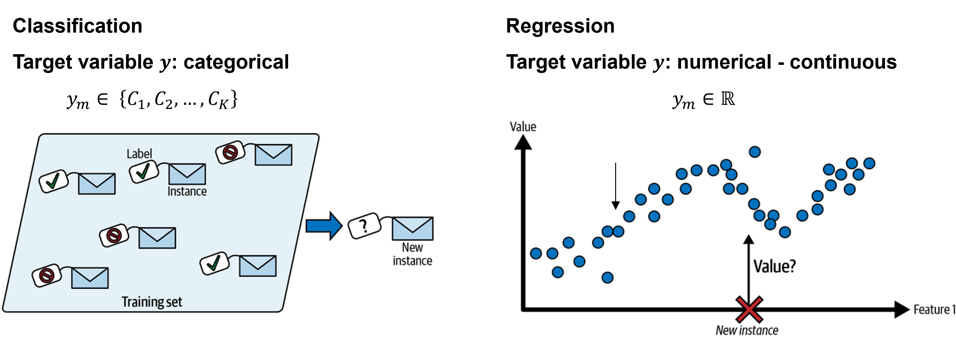
In Classification the target variable is categorical, typically on a nominal scale (the classification algorithms discussed in this course treat ordinally scaled data on a nominal scale). The output values are assumed to belong to a set of discrete classes \(𝑦^{(m)} ∈ \{𝐶_1, 𝐶_2, …, 𝐶_𝐾 \}\)
Example. A spam filter is a good example of this: it is trained with many example emails, along with their corresponding labels pertaining to two classes, “spam” and “no spam” (also called “ham”). The goal is to learn to correctly classify (assign labels to) new emails as spam or ham.
Regression is another supervised learning task, where the goal is to predict a numeric (continuous) target value, i.e. \(y^{(m)} ∈ ℝ\).
Example. A typical regression task is to predict the price of a car from its input features such as mileage, age, brand, etc.
Note that some machine learning methods have variants for both types of tasks, classification and regression.
1.6.2 Evaluating Supervised Machine Learning Models
The ultimate goal in supervised machine learning is to generate predictions for new input samples which are not in the training data. In order to assess the how good the model will perform on this unseen data, we typically estimate it by measuring the quality of the model on a Testset, which contains some data samples that were not used during training of the model.
One way to obtain such a testset is to separat a certain fraction of all labeled data samples (e.g. 20%) and “set it aside”, i.e. split the data into two disjoint subsets: training set and testset. The model is trained on the training set, and once training is finished, we can used the testset to assess the quality of the model in terms of its generalization ability or, in other words, the generalisation error. Since the testset consists of input values and associated expected output values, the output values predicted by the model can be compared with the expected output values and a quality metric which quantitatively measures how well the model’s predictions compare with the expected output values can be calculated. For regression and classification problems different quality metrics are employed, e.g. Mean Squared Error for regression and Accuracy, Precision and Recall for classification.

The evaluation of unsupervised machine learning models is much more difficult due to the more complex nature of the problem.
1.6.3 Supervised Learning Pipeline
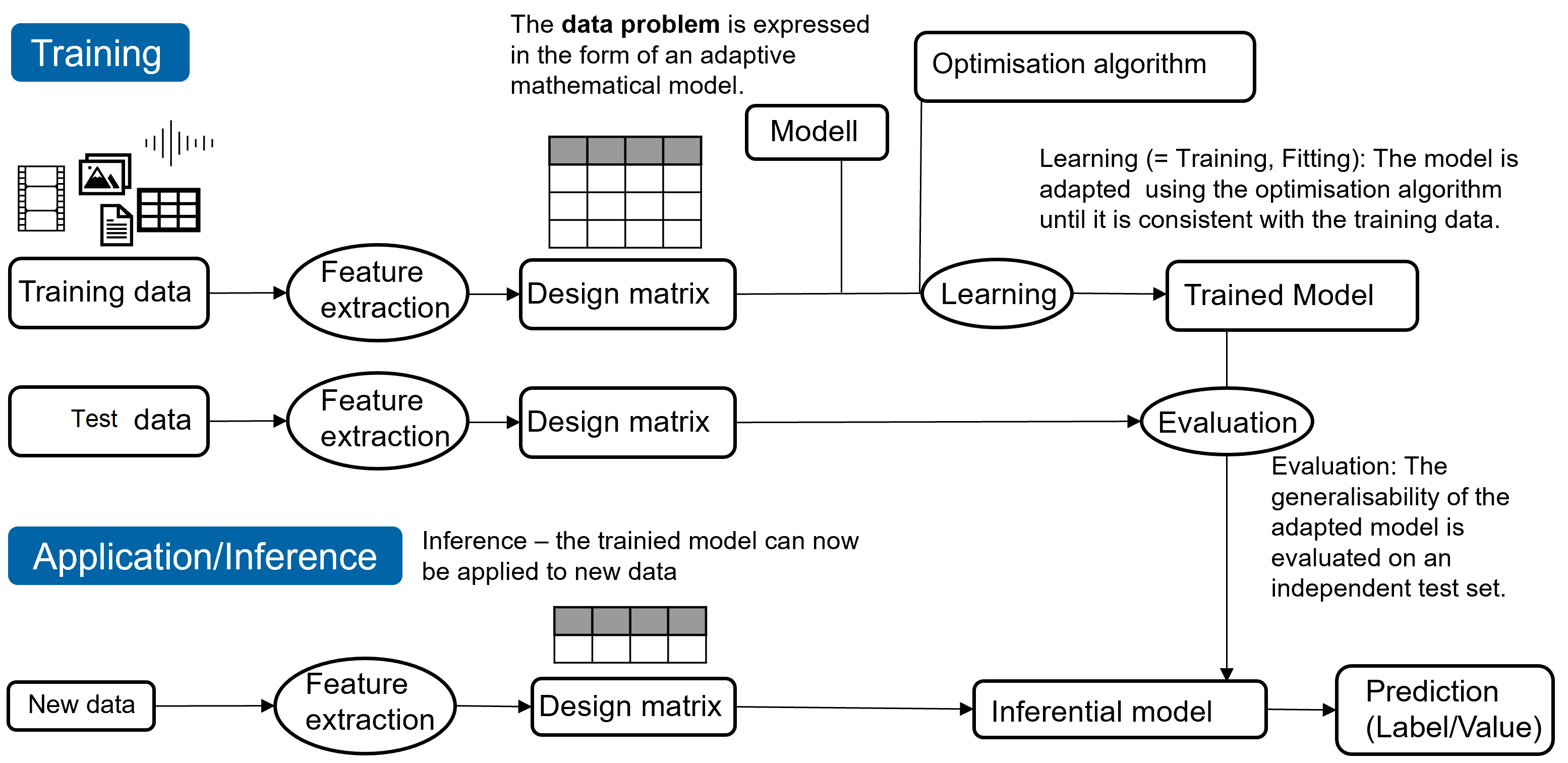
Given a problem (e.g. spam classification) and training data, a typical supervised learning pipeline starts with computing the features for the samples, i.e. representing the data in a structured format. This is stored in the feature matrix, also called the Design Matrix. Then a machine learning algorithm (or model) is selected and trained (learned) on the available training data. More specifically, the model consists of a set of parameters, and these parameters are adjusted using an learning algorithm (in an iterative process) to obtain a consistent mapping between the inputs and their corresponding outputs in the training set. The generalization ability of the final, adapted model (the function determined by the parameter values selected in the learning process) is quantified by computing the estimate of the generalization error on the independent (unseen) testset. The final model can then be applied in practice to predict (infer) the unknown output values for new inputs (e.g. is the email I just received spam or ham). In practice the process above is typically iterated several times, on the one hand, to obtain an machine learning model that gives predictions with sufficient quality to be useful, and on the other hand, to update a deployed model if its performance has dropped due to changes in the data.
